Decision Trees in Machine Learning: Your Path to Mastery

Introduction to Decision Trees in Machine Learning

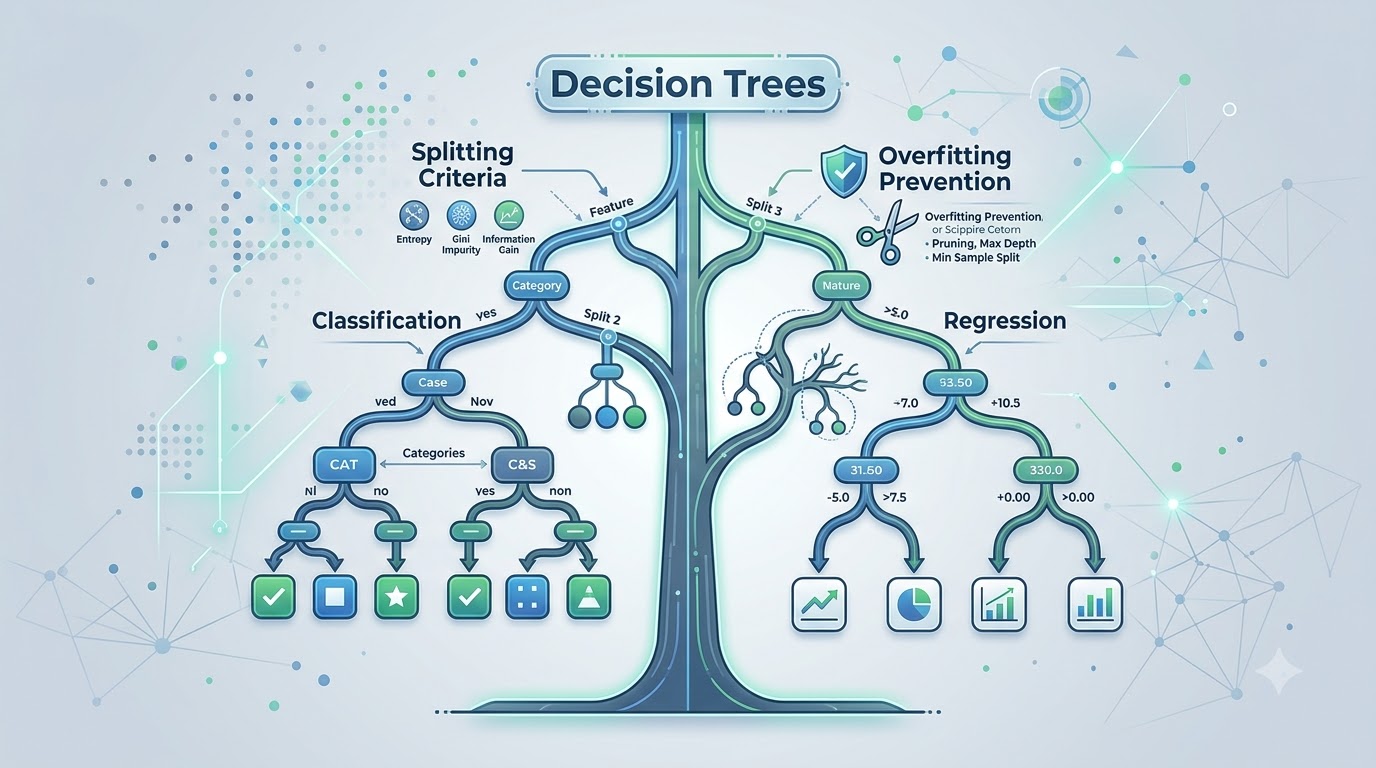
Decision Trees are a fundamental supervised machine learning algorithm. They are versatile, capable of handling both classification and regression problems. Their popularity stems from their intuitive, interpretable, and easily visualizable decision-making process.

These models mimic human decision-making, making them straightforward to understand. They serve as essential building blocks for more complex and powerful ensemble methods like Random Forests and Gradient Boosting.

What Exactly is a Decision Tree?

Imagine you are deciding whether to play outside. You might first check the weather: is it sunny? If yes, you might then check if it's too windy. This step-by-step process is exactly how a Decision Tree works.

A Decision Tree is a flowchart-like structure where each internal node represents a 'test' on an attribute (e.g., 'Is it sunny?'). Each branch represents the outcome of the test, and each leaf node represents a class label (decision) or a numerical value (prediction).

Key components of a Decision Tree include:

• Root Node: The starting point, representing the entire dataset and the initial decision.
• Internal Decision Nodes: Nodes that test a feature and split the data into subsets based on the test's outcome.
• Branches: The connections between nodes, representing the possible outcomes of a decision.
• Leaf Nodes: The terminal nodes of the tree, providing the final classification or prediction.

How Decision Trees Work: The Core Mechanism

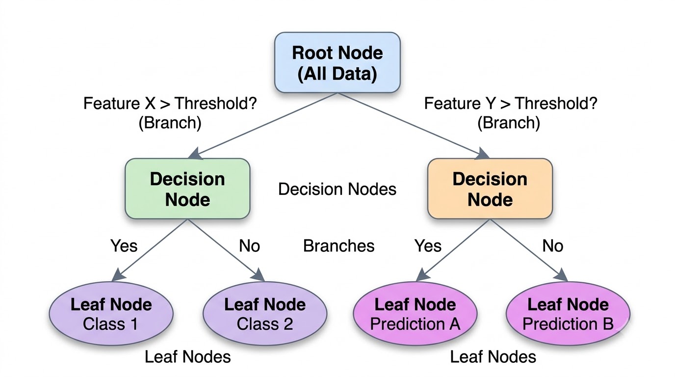
The operational process of a Decision Tree involves recursively partitioning the dataset. The algorithm starts at the root node with the entire dataset. It then evaluates all available features to find the best feature and split point that divides the data into the purest possible subsets.

Consider predicting customer purchase behavior. The tree might first split customers based on 'Age' (e.g., under 30 vs. 30+). Then, within the '30+' group, it might split further based on 'Income' (e.g., high vs. low). This process continues, creating increasingly homogeneous groups until a stopping criterion is met.

The goal at each split is to maximize the homogeneity within the resulting child nodes. This iterative splitting continues until nodes contain mostly one class (for classification) or a narrow range of values (for regression), or until a predefined depth or minimum sample size is reached.

Classification Trees vs. Regression Trees

Decision Trees are powerful because they can tackle both classification and regression problems. The fundamental structure remains the same, but their objectives and how they make predictions differ significantly.

Classification trees are designed to predict a categorical outcome. For example, they might predict whether an email is 'spam' or 'not spam', or if a customer will 'churn' or 'not churn'. The leaf nodes in a classification tree represent the most frequent class within that subset of data.

Regression trees, on the other hand, predict a continuous numerical value. Examples include predicting house prices, stock values, or a patient's recovery time. The leaf nodes in a regression tree typically represent the average or median of the target variable for the data points falling into that leaf.

Key Splitting Criteria: Gini, Entropy, and MSE

At each decision node, the Decision Tree algorithm needs a way to determine the 'best' split. This is where splitting criteria come into play. These metrics quantify how well a particular split separates the data into homogeneous groups.

For classification tasks, common criteria are Gini Impurity and Entropy. Both aim to measure the 'disorder' or 'impurity' of a node. The algorithm seeks to find a split that results in the lowest impurity in the child nodes.

For regression tasks, the primary criterion is Mean Squared Error (MSE). MSE measures the average squared difference between the actual and predicted values. The goal is to find splits that minimize the MSE within the resulting child nodes, leading to more accurate predictions.

Gini Impurity and Entropy Explained in Detail

Gini Impurity measures the probability of incorrectly classifying a randomly chosen element in the dataset if it were randomly labeled according to the distribution of labels in the node. A Gini impurity of 0 means the node is perfectly pure (all elements belong to the same class).

Consider a node with 10 samples: 7 'Yes' and 3 'No'. The Gini impurity would be calculated as 1 - ( (7/10)^2 + (3/10)^2 ) = 1 - (0.49 + 0.09) = 1 - 0.58 = 0.42. The algorithm aims to find splits that reduce this number significantly in the child nodes.

Entropy, derived from information theory, measures the randomness or unpredictability in a node. A node with high entropy is very mixed, while a node with low entropy is more pure. Decision Trees aim to maximize Information Gain, which is the reduction in entropy achieved by a split.

For the same node (7 'Yes', 3 'No'), entropy would be calculated using a logarithmic formula. The split that yields the greatest reduction in entropy (highest Information Gain) is chosen. Both Gini and Entropy generally lead to similar trees, though Gini is computationally faster.

Building a Decision Tree: A Step-by-Step Example

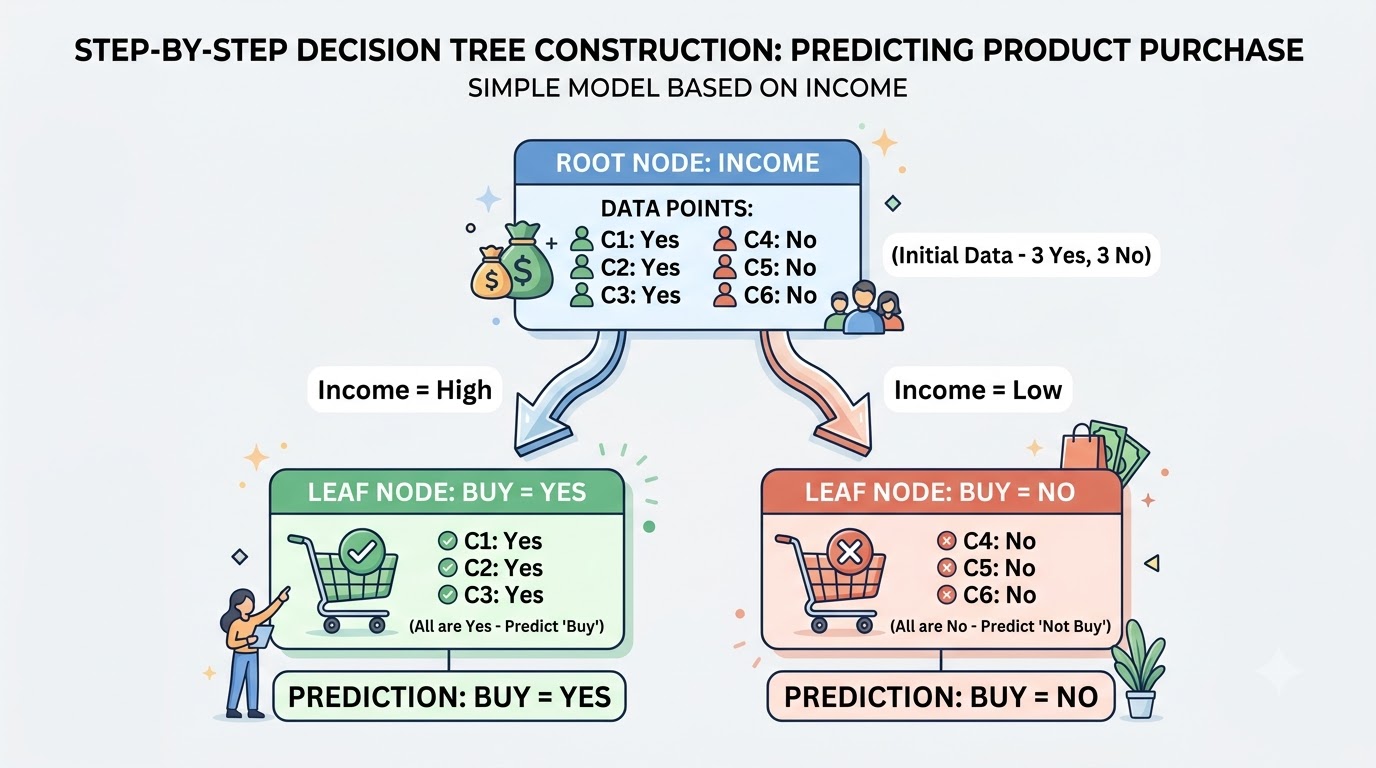
Let's walk through a simplified example to see how a Decision Tree is built. Imagine a tiny dataset for predicting if someone will buy a product based on 'Age' and 'Income'.

Dataset:

• Customer 1: Age=Young, Income=High, Buy=Yes
• Customer 2: Age=Young, Income=Low, Buy=No
• Customer 3: Age=Middle, Income=High, Buy=Yes
• Customer 4: Age=Middle, Income=Low, Buy=No
• Customer 5: Age=Old, Income=High, Buy=Yes
• Customer 6: Age=Old, Income=Low, No

Here's how the tree might be constructed:

1. Step 1: Root Node. The algorithm calculates the impurity (e.g., Gini) for the entire dataset. It then evaluates potential splits based on 'Age' and 'Income'.
2. Step 2: Best Split. Let's say splitting by 'Income' (High vs. Low) yields the highest information gain. 'Income' becomes the root node.
3. Step 3: Branches. Two branches are created: 'Income = High' and 'Income = Low'.
4. Step 4: Child Nodes. The 'Income = High' branch contains (C1, C3, C5) all 'Buy=Yes' (pure). The 'Income = Low' branch contains (C2, C4, C6) all 'Buy=No' (pure).
5. Step 5: Leaf Nodes. Since both child nodes are now pure, they become leaf nodes. The tree building stops.

Addressing Overfitting: Pruning and Hyperparameters

One of the biggest challenges with Decision Trees is overfitting. If allowed to grow without restrictions, a tree can become extremely deep and complex. It might learn the training data too well, including noise and outliers, leading to poor performance on new, unseen data.

To combat overfitting, we employ strategies to control the tree's complexity. These include limiting its growth during construction (pre-pruning) or simplifying it after it's fully grown (post-pruning).

Key concepts for preventing overfitting include: tree depth (maximum number of levels), minimum samples per split (minimum data points required to make a split), and minimum samples per leaf (minimum data points allowed in a terminal node). These act as stopping criteria.

Important Decision Tree Hyperparameters

Hyperparameters are settings that control the learning process and structure of the model. Tuning these parameters is crucial for optimizing a Decision Tree's performance and preventing overfitting or underfitting.

Adjusting these values allows you to find the right balance between model complexity and generalization ability. Understanding their impact is key to building effective Decision Tree models.

Implementing Decision Trees in Python with Scikit-learn

Python's Scikit-learn library provides robust and easy-to-use tools for implementing Decision Trees. We'll walk through a practical example using a classification task. This will cover setting up the environment, preparing data, training the model, making predictions, and visualizing the tree.

Setting Up Your Environment

First, ensure you have the necessary libraries installed. We'll need scikit-learn for the model, pandas for data handling, matplotlib for plotting, and graphviz for tree visualization.

pip install scikit-learn pandas matplotlib graphviz

After installation, import the required modules into your Python script or Jupyter Notebook.

import pandas as pd
from sklearn.datasets import loadᵢris
from sklearn.model_selection import train_test_split
from sklearn.tree import DecisionTreeClassifier, plot_tree
from sklearn.metrics import accuracy_score, classification_report
import matplotlib.pyplot as plt
import graphviz

Data Preparation and Model Training

We'll use the famous Iris dataset, a classic for classification tasks. It contains measurements of iris flowers and their species. We'll load it, split it into features (X) and target (y), and then divide it into training and testing sets.

# Load the Iris dataset
iris = loadᵢris()
X = iris.data
y = iris.target
featureₙames = iris.featureₙames
targetₙames = iris.targetₙames

# Split data into training and testing sets
X_train, X_test, y_train, y_test = train_test_split(X, y, test_size=0.3, random_state=42)

# Initialize the Decision Tree Classifier
# We'll set a max_depth to prevent overfitting and make the tree easier to visualize
dtree_classifier = DecisionTreeClassifier(max_depth=3, random_state=42)

# Train the model on the training data
dtree_classifier.fit(X_train, y_train)

Making Predictions and Evaluation

Once the model is trained, we can use it to make predictions on the unseen test data. We'll then evaluate its performance using common classification metrics like accuracy and a classification report.

# Continued from previous block - requires the setup above

# Make predictions on the test set
y_pred = dtree_classifier.predict(X_test)

# Evaluate the model's performance
accuracy = accuracy_score(y_test, y_pred)
print(f"Accuracy: {accuracy:.2f")

# Display a detailed classification report
print("\nClassification Report:")
print(classification_report(y_test, y_pred, targetₙames=targetₙames))

Visualizing the Trained Decision Tree

Visualizing the Decision Tree is incredibly helpful for understanding its decision-making process. Scikit-learn's plot_tree function allows us to generate a clear graphical representation of the tree. This visualization shows how the model splits data at each node.

# Continued from previous block - requires the setup above

# Plot the Decision Tree
plt.figure(figsize=(15, 10))
plot_tree(dtree_classifier, 
          featureₙames=featureₙames,  
          classₙames=targetₙames, 
          filled=True, 
          rounded=True, 
          fontsize=10)
plt.title("Decision Tree Classifier for Iris Dataset")
plt.show()

# Alternatively, export to Graphviz for more customization (requires Graphviz installation)
# dot_data = export_graphviz(dtree_classifier, out_file=None, 
#                            featureₙames=featureₙames,  
#                            classₙames=targetₙames,  
#                            filled=True, rounded=True,  
#                            special_characters=True)
# graph = graphviz.Source(dot_data)
# graph.render("iris_decision_tree", view=True)

Advantages, Limitations, and Real-World Use Cases

Decision Trees offer a unique blend of simplicity and power, making them a valuable tool in a data scientist's arsenal. However, like all algorithms, they come with their own set of strengths and weaknesses.

Advantages and Limitations of Decision Trees

Decision Trees boast several key advantages:

• Interpretability: Their flowchart-like structure makes them easy to understand and explain, even to non-technical stakeholders.
• Minimal Data Preprocessing: They can handle both numerical and categorical data without extensive scaling or normalization.
• Non-linear Relationships: Capable of capturing complex, non-linear relationships between features and the target variable.
• Feature Selection: Implicitly perform feature selection by prioritizing important features at higher nodes.

However, they also have limitations:

• Overfitting: Prone to overfitting, especially with deep, unrestricted trees, leading to poor generalization.
• Instability: Small changes in the training data can lead to a completely different tree structure.
• Bias with Imbalanced Data: Can be biased towards dominant classes if the dataset is imbalanced.
• Sub-optimality: The greedy approach of finding the best split at each step doesn't guarantee a globally optimal tree.

Real-World Applications of Decision Trees

Decision Trees are widely applied across various industries due to their interpretability and versatility. Here are some prominent examples:

• Customer Churn Prediction: Identifying customers likely to leave a service based on their usage patterns and demographics.
• Loan Approval: Assessing credit risk and deciding whether to approve a loan application.
• Fraud Detection: Flagging suspicious transactions or activities in financial services.
• Medical Diagnosis: Aiding doctors in diagnosing diseases based on patient symptoms and test results.
• Spam Classification: Filtering unwanted emails by analyzing their content and sender characteristics.
• Sales Prediction: Forecasting future sales based on historical data, promotions, and economic indicators.

Their ability to model complex decision paths makes them suitable for problems where understanding the 'why' behind a prediction is as important as the prediction itself.

Decision Trees vs. Linear and Logistic Regression

When choosing a machine learning algorithm, it's essential to understand the strengths of each. Decision Trees differ significantly from linear and logistic regression models in their approach to modeling relationships.

Linear Regression predicts continuous outcomes by fitting a straight line (or hyperplane) to the data. It assumes a linear relationship between features and the target. Logistic Regression, on the other hand, predicts categorical outcomes by modeling the probability of a class using a sigmoid function, also assuming a linear relationship in the log-odds.

Decision Trees do not assume linearity. They partition the feature space into rectangular regions, making them excellent at capturing non-linear interactions and complex decision boundaries. This flexibility comes at the cost of potential overfitting if not properly controlled.

Conclusion: Mastering Decision Trees and Next Steps

Decision Trees are a cornerstone of machine learning, offering an intuitive and powerful way to model complex data. We've explored their core mechanics, from how they split data using criteria like Gini impurity and entropy to their application in both classification and regression tasks.

Understanding the importance of controlling tree complexity through hyperparameters and pruning is crucial for building robust models that generalize well. Their interpretability makes them invaluable for scenarios where understanding the decision process is as important as the prediction itself.

As a natural next step in your machine learning journey, consider exploring ensemble methods. Algorithms like Random Forests and Gradient Boosting build upon the foundation of Decision Trees to achieve even higher accuracy and robustness, mitigating many of the limitations of a single tree.