Python Supervised Learning: Classify vs Regress Guide

Introduction to Supervised Learning: Classification and Regression

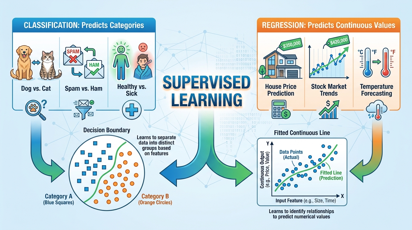
Supervised learning stands as a cornerstone of modern machine learning, forming the basis for countless applications that impact our daily lives, from personalized recommendations to medical diagnostics. At its heart, supervised learning involves training a model on a labeled dataset, where each input example is paired with its correct output.

This 'supervision' allows the model to learn the underlying patterns and relationships between features and targets, enabling it to make accurate predictions on new, unseen data. Within this powerful paradigm, two fundamental categories emerge: classification and regression. While both aim to predict outcomes, they tackle distinct types of problems. Classification models are designed to predict discrete, categorical labels, such as identifying whether an email is spam or not, or classifying an image as a 'cat' or 'dog'. In contrast, regression models focus on predicting continuous numerical values, like forecasting house prices, predicting stock market trends, or estimating a patient's recovery time.

Understanding the nuanced differences between classification and regression is not merely an academic exercise; it is absolutely crucial for any aspiring or experienced machine learning practitioner. The choice between these two approaches dictates everything from the selection of appropriate algorithms and the preprocessing steps applied to the data, to the metrics used for evaluating model performance and, ultimately, the success and reliability of the deployed solution. A clear grasp of these distinctions empowers developers to frame problems correctly, choose the most suitable tools, and build robust, effective machine learning systems that deliver real-world value.

What is Supervised Learning?

Supervised learning is a machine learning approach characterized by its reliance on labeled datasets. In this context, 'labeled' means that for every input data point, there is a corresponding correct output or 'target' value. Think of it like a student learning with a teacher: the teacher provides examples (input data) along with the correct answers (labels), and the student learns to associate the inputs with their respective outputs.

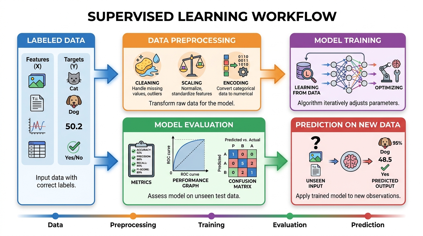
For instance, if you're building a model to identify images of cats, your dataset would consist of numerous images (inputs) each explicitly labeled as either 'cat' or 'not cat' (outputs). The primary goal of supervised learning is for the model to learn a mapping function from the input features to the target variable, such that it can accurately predict the output for new, unseen inputs. The typical workflow for a supervised learning project begins with meticulous data preparation, which involves collecting, cleaning, and transforming raw data into a suitable format.

This often includes handling missing values, encoding categorical features, and scaling numerical data. Next, the prepared dataset is split into training and testing (and sometimes validation) sets. The model is then trained on the training data, where it iteratively adjusts its internal parameters to minimize the difference between its predictions and the actual labels. After training, the model's performance is evaluated on the unseen test data to assess its generalization ability. Finally, once validated, the trained model can be deployed to make predictions on real-world, new data, providing insights or automating decisions based on the patterns it has learned.

What is Classification?

Classification is a fundamental supervised learning task where the objective is to predict a categorical label or class for a given input. Unlike regression, which deals with continuous values, classification models output discrete categories. Imagine you have a set of emails, and you want to determine if an incoming email is 'spam' or 'not spam'; this is a classic classification problem.

The model learns from historical emails that have already been labeled as spam or not and then applies that learned knowledge to new emails. Classification problems can be broadly categorized into several types: Binary Classification involves predicting one of two possible classes (e.g., yes/no, true/false, spam/not spam). Multi-class Classification extends this to more than two classes, where each input belongs to exactly one class (e.g., classifying images of fruits into 'apple', 'banana', 'orange'). Multi-label Classification is a more complex scenario where an input can belong to multiple classes simultaneously (e.g., an image might contain both a 'dog' and a 'cat').

Practical applications of classification are ubiquitous across various industries. In healthcare, it's used for disease diagnosis (e.g., predicting if a tumor is malignant or benign) or identifying high-risk patients. In finance, classification models detect fraudulent transactions or assess credit risk. For natural language processing, sentiment analysis (classifying text as positive, negative, or neutral) and spam detection are prime examples. Even in computer vision, object recognition and image categorization rely heavily on classification techniques. The core idea remains consistent: assigning an input to one or more predefined categories based on its features.

Common Classification Algorithms

A diverse array of algorithms has been developed to tackle classification problems, each with its unique approach to learning decision boundaries and making predictions. Choosing the right algorithm often depends on the nature of your data, the complexity of the problem, and the interpretability requirements. Here are some of the most commonly used classification algorithms:

• Logistic Regression: Despite its name, Logistic Regression is a powerful classification algorithm. It models the probability of a binary outcome using a logistic sigmoid function. It's simple, efficient, and highly interpretable, making it a great baseline model. Its strength lies in its speed and ability to provide probability scores, but it assumes a linear relationship between features and the log-odds of the outcome, which might not hold for complex, non-linear data. It's often used for spam detection, credit scoring, and medical diagnosis.
• Decision Trees: Decision Trees work by recursively splitting the dataset into subsets based on the most significant features, creating a tree-like structure of decisions. They are intuitive, easy to visualize, and can handle both numerical and categorical data without extensive preprocessing. However, individual decision trees can be prone to overfitting, especially with deep trees, and can be unstable to small variations in data. They are excellent for problems requiring interpretability, such as customer churn prediction or medical decision support systems.
• Support Vector Machines (SVM): SVMs aim to find the optimal hyperplane that best separates different classes in the feature space, maximizing the margin between the closest data points (support vectors) of each class. They are highly effective in high-dimensional spaces and can handle non-linear relationships using various kernel functions (e.g., RBF, polynomial). SVMs can be computationally intensive for large datasets and less interpretable than simpler models. They are widely used in image classification, text categorization, and bioinformatics.
• K-Nearest Neighbors (KNN): KNN is a non-parametric, instance-based learning algorithm that classifies a new data point based on the majority class of its 'k' nearest neighbors in the feature space. It's simple to understand and implement, and it adapts well to complex decision boundaries. The main drawbacks include its computational cost for large datasets (as it needs to store all training data) and its sensitivity to the choice of 'k' and the distance metric. KNN is often applied in recommendation systems, pattern recognition, and anomaly detection.
• Random Forest: An ensemble learning method, Random Forest builds multiple decision trees during training and outputs the class that is the mode of the classes (classification) or mean prediction (regression) of the individual trees. It significantly reduces overfitting compared to single decision trees and generally provides higher accuracy. It's robust to noisy data and can handle a large number of features. While powerful, it can be less interpretable than a single decision tree and computationally more expensive. It's a go-to algorithm for many tasks, including fraud detection, medical image analysis, and predicting customer behavior.

Classification Evaluation Metrics

Once a classification model is trained, evaluating its performance is critical to understand how well it generalizes to unseen data and to ensure it meets the problem's objectives. A single metric rarely tells the whole story, and different metrics are suitable for different scenarios, especially when dealing with imbalanced datasets.

• Accuracy: This is the most straightforward metric, calculated as the ratio of correctly predicted observations to the total observations. While easy to understand, accuracy can be misleading for imbalanced datasets. For example, if 95% of your data belongs to one class, a model that always predicts that class will have 95% accuracy but be useless.
• Confusion Matrix: A confusion matrix is a table that describes the performance of a classification model on a set of test data for which the true values are known. It breaks down predictions into four categories:
  • True Positives (TP): Correctly predicted positive class.
  • True Negatives (TN): Correctly predicted negative class.
  • False Positives (FP): Incorrectly predicted positive class (Type I error).
  • False Negatives (FN): Incorrectly predicted negative class (Type II error).

The confusion matrix forms the basis for calculating other metrics.

• Precision: Precision measures the proportion of positive identifications that were actually correct. It's calculated as TP / (TP + FP). High precision indicates a low false positive rate. It's crucial when the cost of a false positive is high (e.g., spam detection, where legitimate emails shouldn't be marked as spam).
• Recall (Sensitivity): Recall measures the proportion of actual positives that were correctly identified. It's calculated as TP / (TP + FN). High recall indicates a low false negative rate. It's important when the cost of a false negative is high (e.g., medical diagnosis, where missing a disease is critical).
• F1-Score: The F1-Score is the harmonic mean of Precision and Recall. It provides a single score that balances both metrics, making it particularly useful when you need to consider both false positives and false negatives, especially with uneven class distributions. It's calculated as 2 (Precision Recall) / (Precision + Recall).
• ROC Curve and AUC (Area Under the Curve): The Receiver Operating Characteristic (ROC) curve is a plot that illustrates the diagnostic ability of a binary classifier system as its discrimination threshold is varied. It plots the True Positive Rate (Recall) against the False Positive Rate (1 - Specificity) at various threshold settings. The Area Under the ROC Curve (AUC) provides a single scalar value that summarizes the overall performance across all possible classification thresholds. An AUC of 1.0 indicates a perfect classifier, while 0.5 indicates a random classifier. AUC is robust to class imbalance and is excellent for comparing different models.

Classification Example in Python with Scikit-learn

Let's put theory into practice by building a complete classification model using Python and the widely-used Scikit-learn library. We'll use the famous Iris dataset, a classic for multi-class classification, to predict the species of iris flower based on its sepal and petal measurements. This example will walk through data loading, splitting, model training with Logistic Regression, making predictions, and evaluating the model's performance using the metrics we just discussed. The goal is to provide a clear, runnable example that you can adapt for your own classification tasks.

We'll start by importing the necessary libraries, then load the dataset, prepare it for training by splitting into features and target, and then divide it into training and testing sets to ensure our model's evaluation is unbiased. Finally, we'll train a Logistic Regression model, make predictions on the test set, and print out a classification report and confusion matrix to assess its effectiveness. This hands-on approach will solidify your understanding of the classification pipeline.

# Import necessary libraries
import numpy as np
import pandas as pd
from sklearn.datasets import load_iris
from sklearn.model_selection import train_test_split
from sklearn.linear_model import LogisticRegression
from sklearn.metrics import classification_report, confusion_matrix, accuracy_score
import matplotlib.pyplot as plt
import seaborn as sns

# Load the Iris dataset
# The Iris dataset is a classic multi-class classification dataset.
# It contains 150 samples of iris flowers, with 4 features and 3 target classes (species).
iris = load_iris()
X = iris.data  # Features (sepal length, sepal width, petal length, petal width)
y = iris.target # Target (species: 0, 1, 2 representing setosa, versicolor, virginica)

# Display basic information about the dataset
print("Features shape:", X.shape)
print("Target shape:", y.shape)
print("Target names:", iris.target_names)

# Split the dataset into training and testing sets
# We use 80% of the data for training and 20% for testing.
# stratify=y ensures that the proportion of target classes is the same in both train and test sets.
# random_state for reproducibility.
X_train, X_test, y_train, y_test = train_test_split(X, y, test_size=0.2, random_state=42, stratify=y)

print(f"Training set size: {X_train.shape[0]} samples")
print(f"Testing set size: {X_test.shape[0]} samples")

# Initialize and train a Logistic Regression model
# Logistic Regression is a good baseline for classification tasks.
# max_iter is increased to ensure convergence for some datasets.
model = LogisticRegression(max_iter=200, random_state=42)
model.fit(X_train, y_train)

# Make predictions on the test set
y_pred = model.predict(X_test)

# Evaluate the model's performance
print("\n--- Model Evaluation ---")

# Accuracy Score
accuracy = accuracy_score(y_test, y_pred)
print(f"Accuracy: {accuracy:.4f}")

# Classification Report
# Provides precision, recall, f1-score, and support for each class.
print("\nClassification Report:")
print(classification_report(y_test, y_pred, target_names=iris.target_names))

# Confusion Matrix
# Visualizes the performance of an algorithm, showing true vs. predicted labels.
cm = confusion_matrix(y_test, y_pred)
print("\nConfusion Matrix:")
print(cm)

# Plotting the Confusion Matrix for better visualization
plt.figure(figsize=(8, 6))
sns.heatmap(cm, annot=True, fmt='d', cmap='Blues',
            xticklabels=iris.target_names, yticklabels=iris.target_names)
plt.xlabel('Predicted Label')
plt.ylabel('True Label')
plt.title('Confusion Matrix for Iris Classification')
plt.show()

# Example of predicting a single new sample (hypothetical)
# Let's create a dummy new sample with 4 features
new_sample = np.array([[5.1, 3.5, 1.4, 0.2]]) # Features similar to Iris setosa
predicted_species_idx = model.predict(new_sample)[0]
predicted_species_name = iris.target_names[predicted_species_idx]
print(f"\nPredicted species for new sample {new_sample[0]}: {predicted_species_name}")

# Get prediction probabilities for the new sample
predicted_probabilities = model.predict_proba(new_sample)[0]
print(f"Prediction probabilities for new sample: {predicted_probabilities}")
for i, prob in enumerate(predicted_probabilities):
    print(f"  {iris.target_names[i]}: {prob:.4f}")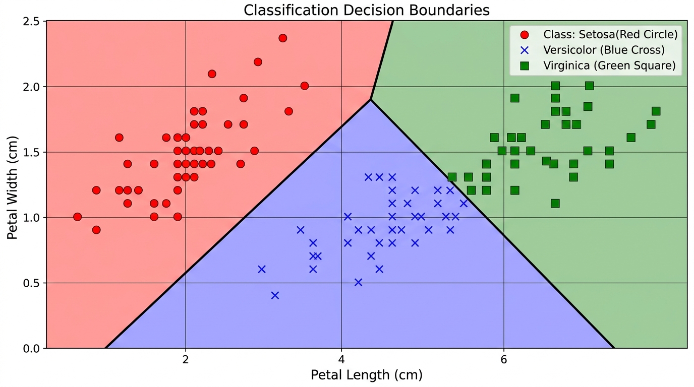

Visualizing Classification Decision Boundaries

What is Regression?

Regression, another cornerstone of supervised learning, focuses on predicting continuous numerical values rather than discrete categories. While classification answers 'what kind?' or 'which group?', regression answers 'how much?' or 'how many?'. The goal of a regression model is to estimate a target variable that is a real number, such as predicting the price of a house, forecasting stock market fluctuations, or determining the optimal dosage of a drug. The model learns the relationship between input features and a continuous output by analyzing historical data where both features and the actual continuous target values are known.

There are several types of regression problems, each suited for different data patterns. Simple Linear Regression involves predicting a single continuous output based on a single input feature, assuming a linear relationship. Multiple Linear Regression extends this to multiple input features. Polynomial Regression allows for non-linear relationships by fitting a polynomial equation to the data. Other advanced forms include Ridge, Lasso, and Elastic Net Regression, which incorporate regularization techniques to prevent overfitting.

Real-world applications of regression are vast and impactful. In economics, it's used for predicting GDP growth or inflation rates. Environmental science employs regression to forecast weather patterns or model pollution levels. In business, it helps in sales forecasting, predicting customer lifetime value, or optimizing pricing strategies. Manufacturing uses regression for predictive maintenance, estimating equipment wear and tear. The ability to accurately predict continuous outcomes provides invaluable insights for decision-making across virtually every industry.

Common Regression Algorithms

Just as with classification, a variety of algorithms are available for regression tasks, each with its own mathematical foundation and suitability for different types of data and problems. Understanding these algorithms helps in selecting the most effective tool for your specific predictive modeling needs.

• Linear Regression: This is perhaps the simplest and most fundamental regression algorithm. It models the relationship between a dependent variable and one or more independent variables by fitting a linear equation to the observed data. The goal is to find the line (or hyperplane in higher dimensions) that minimizes the sum of squared differences between the observed and predicted values. Linear Regression is highly interpretable and computationally efficient. Its main limitation is the assumption of linearity between features and the target, making it less effective for complex, non-linear relationships. It's widely used for predicting sales, forecasting trends, and simple statistical modeling.
• Polynomial Regression: An extension of linear regression, Polynomial Regression models the relationship between the independent variable and the dependent variable as an nth-degree polynomial. This allows it to fit a much wider range of curves and capture non-linear relationships that simple linear regression cannot. While more flexible, it can be prone to overfitting, especially with high-degree polynomials, and interpretability decreases with increasing complexity. It's useful when the relationship between variables is clearly curvilinear, such as modeling growth rates or physical phenomena.
• Ridge and Lasso Regression (Regularized Regression): These are extensions of linear regression that introduce regularization terms to the cost function. Regularization helps prevent overfitting by penalizing large coefficients.
  • Ridge Regression (L2 regularization) adds a penalty equal to the square of the magnitude of coefficients. It shrinks coefficients towards zero but rarely makes them exactly zero.
  • Lasso Regression (L1 regularization) adds a penalty equal to the absolute value of the magnitude of coefficients. It can shrink some coefficients to exactly zero, effectively performing feature selection.

Both are excellent for handling multicollinearity and improving generalization performance, especially with many features. They are widely used in genomics, finance, and any domain where feature selection or robust models are needed.

• Decision Tree Regressor: Similar to its classification counterpart, a Decision Tree Regressor splits the data into branches based on feature values, but instead of predicting a class, it predicts a continuous value by taking the average of the target values in the leaf nodes. They are easy to understand, visualize, and can capture complex non-linear relationships. Like classification trees, they can suffer from overfitting and instability. They are useful for problems where feature interactions are important and interpretability is desired, such as predicting customer spending or property values.
• Random Forest Regressor: An ensemble method that builds multiple decision tree regressors and averages their individual predictions to produce a more robust and accurate forecast. It significantly reduces the risk of overfitting inherent in single decision trees and generally provides higher predictive accuracy. Random Forest Regressors are robust to noisy data, can handle a large number of features, and provide feature importance scores. They are a powerful choice for complex regression tasks, including stock price prediction, energy consumption forecasting, and predicting biological responses.

Regression Evaluation Metrics

Evaluating the performance of a regression model requires different metrics than those used for classification, as we are dealing with continuous predictions rather than discrete categories. The goal is to quantify how close the model's predictions are to the actual observed values.

• Mean Absolute Error (MAE): MAE is the average of the absolute differences between the predicted and actual values. It measures the average magnitude of the errors in a set of predictions, without considering their direction. MAE is robust to outliers because it doesn't square the errors, making it a good choice when you want to understand the typical error magnitude in the same units as the target variable. It's calculated as (1/n) * sum(|actual - predicted|).
• Mean Squared Error (MSE): MSE is the average of the squared differences between the predicted and actual values. By squaring the errors, MSE penalizes larger errors more heavily than smaller ones, making it sensitive to outliers. This can be beneficial if large errors are particularly undesirable. However, its units are squared, which can make interpretation less intuitive than MAE. It's calculated as (1/n) * sum((actual - predicted)^2).
• Root Mean Squared Error (RMSE): RMSE is the square root of the MSE. It brings the error metric back into the same units as the target variable, making it more interpretable than MSE. Like MSE, it penalizes large errors more, making it sensitive to outliers. RMSE is one of the most commonly used regression metrics, especially when the target variable has a wide range of values. It's calculated as sqrt(MSE).
• R-squared (R2 Score): R-squared, also known as the coefficient of determination, measures the proportion of the variance in the dependent variable that can be predicted from the independent variables. It provides an indication of how well the model fits the observed data. An R-squared value of 1 indicates that the model perfectly predicts the target variable, while 0 indicates that the model explains none of the variance. A negative R-squared means the model is worse than simply predicting the mean of the target variable. It's a relative measure and is useful for comparing models, but it can be misleading if not interpreted carefully, as adding more features can increase R-squared even if they don't improve the model's generalization. It's calculated as 1 - (sum((actual - predicted)^2) / sum((actual - mean_actual)^2)).

Choosing the right metric depends on the specific problem and the implications of different types of errors. For instance, if outliers are critical, MSE/RMSE might be preferred; if interpretability in original units is key, MAE is better; and if you need a relative measure of fit, R-squared is valuable.

Regression Example in Python with Scikit-learn

Now, let's dive into a practical regression example using Python and Scikit-learn. We'll use a synthetic dataset for simplicity, which allows us to clearly visualize the linear relationship and the model's fit. The goal is to predict a continuous target variable based on one or more input features. This example will cover the essential steps: generating a dataset, splitting it into training and testing sets, training a Linear Regression model, making predictions, and evaluating its performance using the regression metrics we just discussed.

We will also visualize the regression line to intuitively understand how well our model captures the underlying trend in the data. This hands-on demonstration will provide a solid foundation for applying regression techniques to your own continuous prediction problems. We'll start by creating some synthetic data that exhibits a clear linear trend with some added noise, mimicking real-world data. Then, we'll follow the standard machine learning pipeline: splitting the data, training a LinearRegression model, making predictions, and finally, calculating MAE, MSE, RMSE, and R-squared to quantify the model's accuracy. Visualizing the actual versus predicted values will offer a qualitative assessment of the model's fit.

# Import necessary libraries
import numpy as np
import pandas as pd
from sklearn.model_selection import train_test_split
from sklearn.linear_model import LinearRegression
from sklearn.metrics import mean_absolute_error, mean_squared_error, r2_score
import matplotlib.pyplot as plt
import seaborn as sns

# Generate a synthetic dataset for regression
# We'll create a simple linear relationship with some random noise.
np.random.seed(42) # for reproducibility
X = 2 * np.random.rand(100, 1) # 100 samples, 1 feature
y = 4 + 3 * X + np.random.randn(100, 1) # y = 4 + 3x + noise

# Display basic information about the synthetic dataset
print("Features shape:", X.shape)
print("Target shape:", y.shape)

# Plot the synthetic data to visualize the relationship
plt.figure(figsize=(10, 6))
plt.scatter(X, y, color='blue', label='Actual Data Points')
plt.xlabel('Feature (X)')
plt.ylabel('Target (y)')
plt.title('Synthetic Regression Dataset')
plt.legend()
plt.grid(True)
plt.show()

# Split the dataset into training and testing sets
# We use 80% of the data for training and 20% for testing.
X_train, X_test, y_train, y_test = train_test_split(X, y, test_size=0.2, random_state=42)

print(f"Training set size: {X_train.shape[0]} samples")
print(f"Testing set size: {X_test.shape[0]} samples")

# Initialize and train a Linear Regression model
model = LinearRegression()
model.fit(X_train, y_train)

# Make predictions on the test set
y_pred = model.predict(X_test)

# Evaluate the model's performance
print("\n--- Model Evaluation ---")

# Mean Absolute Error (MAE)
mae = mean_absolute_error(y_test, y_pred)
print(f"Mean Absolute Error (MAE): {mae:.4f}")

# Mean Squared Error (MSE)
mse = mean_squared_error(y_test, y_pred)
print(f"Mean Squared Error (MSE): {mse:.4f}")

# Root Mean Squared Error (RMSE)
rmse = np.sqrt(mse)
print(f"Root Mean Squared Error (RMSE): {rmse:.4f}")

# R-squared (R2 Score)
r2 = r2_score(y_test, y_pred)
print(f"R-squared (R2 Score): {r2:.4f}")

# Print model coefficients
print(f"\nModel Intercept: {model.intercept_[0]:.4f}")
print(f"Model Coefficient (slope): {model.coef_[0][0]:.4f}")

# Visualize the regression line fit
plt.figure(figsize=(10, 6))
plt.scatter(X_test, y_test, color='blue', label='Actual Test Data')
plt.plot(X_test, y_pred, color='red', linewidth=2, label='Regression Line (Predictions)')
plt.xlabel('Feature (X)')
plt.ylabel('Target (y)')
plt.title('Linear Regression: Actual vs. Predicted Values')
plt.legend()
plt.grid(True)
plt.show()

# Example of predicting a single new sample (hypothetical)
new_sample_X = np.array([[1.5]]) # A new feature value
predicted_y = model.predict(new_sample_X)[0][0]
print(f"\nPredicted target for new sample X={new_sample_X[0][0]}: {predicted_y:.4f}")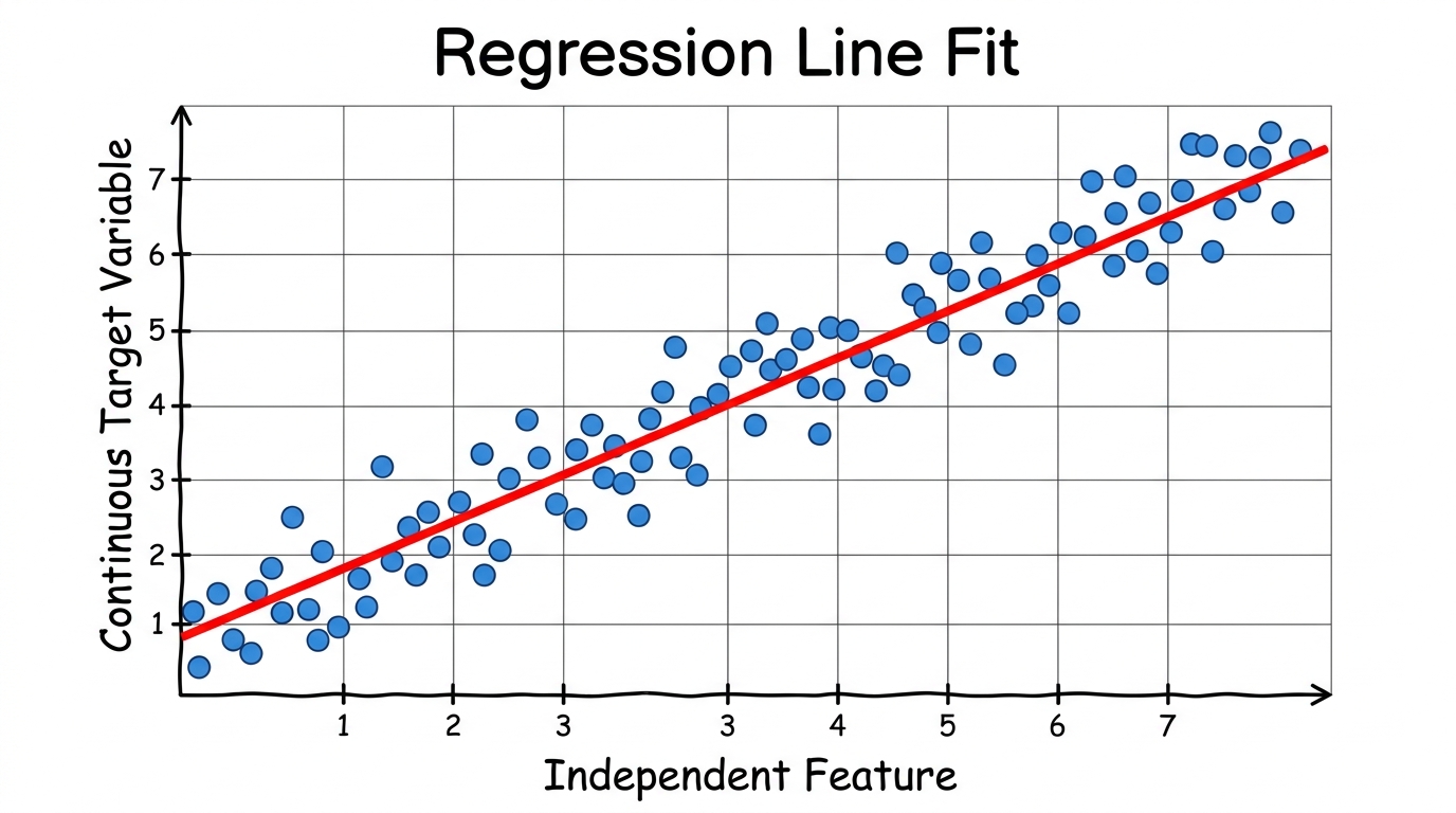

Visualizing Regression Line Fit

Classification vs Regression: Key Differences

While both classification and regression fall under the umbrella of supervised learning, their fundamental objectives and the nature of their outputs are distinctly different. Understanding these core differences is paramount for correctly framing a machine learning problem and selecting the appropriate tools and techniques. Misidentifying a problem as classification when it's truly regression (or vice-versa) can lead to ineffective models and misleading results.

The distinction primarily lies in the type of variable they aim to predict. Classification deals with discrete, categorical outcomes, essentially putting data points into predefined bins or groups. Regression, on the other hand, is concerned with predicting a continuous, numerical value, estimating a point along a spectrum. This fundamental difference cascades into every aspect of the machine learning pipeline, from the algorithms employed to the metrics used for evaluating success.

For instance, an algorithm like Logistic Regression, despite its name, is a classifier because it predicts probabilities of belonging to a class, which are then thresholded to yield a discrete label. Conversely, a Decision Tree can be adapted for both classification (predicting the most frequent class in a leaf) and regression (predicting the average value in a leaf). The choice of evaluation metrics is also a direct consequence of the problem type; accuracy and F1-score are meaningless for regression, just as MAE and R-squared are irrelevant for classification. The following table provides a comprehensive comparison of these two vital supervised learning paradigms.

How to Choose Between Classification and Regression

The critical first step in any supervised machine learning project is to correctly identify whether the problem at hand is a classification or a regression task. This decision fundamentally shapes your entire approach, from data preparation to model selection and evaluation. The primary determinant for this choice is the nature of your target variable – the outcome you are trying to predict.

• Analyze the Target Variable:
  • If your target variable represents distinct, finite categories or labels, then it's a classification problem. Examples include 'yes' or 'no', 'true' or 'false', 'spam' or 'not spam', different types of diseases, or various animal species. The output is a class label.
  • If your target variable is a continuous numerical value that can take any value within a range, then it's a regression problem. Examples include house prices, temperature, stock values, age, or sales figures. The output is a quantity.
• Consider the Business Objective: Beyond the data type, think about what the business or application needs to achieve.
  • Do you need to categorize items, make a binary decision, or assign a label? This points to classification. For instance, 'Is this customer likely to churn?' (binary classification) or 'Which product category does this new item belong to?' (multi-class classification).
  • Do you need to estimate a quantity, forecast a future value, or predict a magnitude? This indicates regression. For example, 'What will be the sales revenue next quarter?' or 'How many units will be sold next month?'.
• Expected Output Type: What kind of output do you expect from your model?
  • If the desired output is a discrete choice or group, use classification.
  • If the desired output is a numerical value on a scale, use regression.

It's important to note that sometimes a problem can be framed in both ways. For example, predicting a person's age could be a regression task (predicting the exact age) or a classification task (predicting age groups like 'child', 'teenager', 'adult'). The choice depends entirely on the specific question you're trying to answer and the utility of the output for your application. Always start by clearly defining your problem statement and the nature of the outcome you wish to predict.

Real-World Applications of Classification and Regression

The theoretical distinctions between classification and regression become vividly clear when we look at their widespread applications across numerous industries. These supervised learning techniques power many of the intelligent systems we interact with daily, often without even realizing it.

• Healthcare:
  • Classification: Disease diagnosis (e.g., predicting if a patient has cancer based on medical images or lab results), identifying high-risk patients for certain conditions, drug efficacy prediction (e.g., will a drug work for a specific patient profile).
  • Regression: Predicting patient recovery time after surgery, optimizing drug dosages based on patient characteristics, forecasting hospital bed occupancy, estimating the cost of medical treatments.
• Finance:
  • Classification: Fraud detection (e.g., flagging suspicious credit card transactions), credit risk assessment (e.g., determining if a loan applicant is likely to default), stock market trend prediction (e.g., will a stock go up or down).
  • Regression: Stock price forecasting, predicting future interest rates, estimating property values for mortgages, calculating customer lifetime value.
• E-commerce and Marketing:
  • Classification: Customer churn prediction (identifying customers likely to leave), sentiment analysis of product reviews, targeted advertising (e.g., classifying users into segments for specific ads), recommendation systems (e.g., predicting if a user will like a product).
  • Regression: Sales forecasting, predicting customer spending, optimizing pricing strategies, estimating website traffic, predicting conversion rates.
• Cybersecurity:
  • Classification: Intrusion detection (identifying malicious network activity), malware classification (categorizing types of malicious software), phishing email detection.
  • Regression: Predicting the severity of a cyber-attack, forecasting the number of security incidents over time.
• Manufacturing and Industrial:
  • Classification: Quality control (e.g., classifying products as defective or non-defective), anomaly detection in sensor data for equipment failure.
  • Regression: Predictive maintenance (estimating remaining useful life of machinery), optimizing production parameters, forecasting energy consumption.
• Environmental Science:
  • Classification: Classifying land use from satellite imagery, identifying species from environmental data.
  • Regression: Predicting air pollution levels, forecasting weather conditions (temperature, rainfall), modeling climate change impacts.

These examples underscore the versatility and power of supervised learning, demonstrating how these techniques are instrumental in solving complex, real-world problems by extracting meaningful insights from data.

Common Mistakes to Avoid in Supervised Learning

Building effective supervised learning models is as much about knowing what to do as it is about knowing what to avoid. Many common pitfalls can derail a project, leading to inaccurate models, wasted effort, and poor decision-making. Being aware of these mistakes can significantly improve the robustness and reliability of your machine learning solutions.

• Incorrect Problem Framing: One of the most fundamental errors is misclassifying a problem as regression when it's classification, or vice-versa. For example, trying to predict discrete customer segments with a regression model will yield nonsensical results. Always ensure your target variable's nature aligns with the chosen supervised learning paradigm.
• Choosing an Inappropriate Algorithm: Not all algorithms are created equal, and each has its strengths and weaknesses. Using a simple linear model for highly non-linear data, or a complex deep learning model for a small, simple dataset, can lead to suboptimal performance. Understand the assumptions and capabilities of different algorithms before applying them.
• Misinterpreting Evaluation Metrics: Relying solely on accuracy for imbalanced classification problems, or using MSE when MAE is more interpretable for outliers in regression, can lead to flawed conclusions. Always select metrics that align with the business objective and the characteristics of your data. Understand what each metric truly represents.
• Data Leakage: This is a subtle but critical error where information from the test set "leaks" into the training set, leading to overly optimistic performance estimates. This can happen through improper data preprocessing (e.g., scaling the entire dataset before splitting) or using features that are derived from the target variable in a way that wouldn't be available at prediction time. Always split your data before any data transformation steps that learn parameters from the data.
• Overfitting and Underfitting:
  • Overfitting occurs when a model learns the training data too well, including its noise and specific patterns, and fails to generalize to new, unseen data. The model performs excellently on the training set but poorly on the test set.
  • Underfitting occurs when a model is too simple to capture the underlying patterns in the data, performing poorly on both training and test sets.

Both are common and require careful tuning of model complexity, regularization, and feature engineering.

• Ignoring Feature Scaling: Many machine learning algorithms (e.g., SVMs, KNN, Logistic Regression, Neural Networks) are sensitive to the scale of input features. Features with larger ranges can dominate the distance calculations or gradient descent updates. Failing to scale features (e.g., using StandardScaler or MinMaxScaler) can lead to slower convergence or suboptimal model performance.
• Improper Data Splitting: Not splitting data into distinct training, validation, and test sets, or using a non-random split that introduces bias, can lead to unreliable performance estimates. Cross-validation is a robust technique to get a more reliable estimate of model performance and reduce variance.

Avoiding these common mistakes requires a systematic approach, a deep understanding of your data, and continuous experimentation and validation throughout the machine learning lifecycle.

Best Practices for Supervised Learning Models

To build robust, reliable, and high-performing supervised learning models, it's essential to follow a set of best practices that span the entire machine learning pipeline. These practices help mitigate common pitfalls and ensure that your models are not only accurate but also generalizable and maintainable.

• Thorough Data Preprocessing and Cleaning: This is arguably the most crucial step.
  • Handle Missing Values: Impute missing data using appropriate strategies (mean, median, mode, advanced imputation techniques) or remove rows/columns if necessary.
  • Encode Categorical Features: Convert categorical data into numerical formats using techniques like One-Hot Encoding or Label Encoding.
  • Scale Numerical Features: Apply standardization (e.g., StandardScaler) or normalization (e.g., MinMaxScaler) to numerical features, especially for algorithms sensitive to feature scales.
  • Outlier Detection and Treatment: Identify and appropriately handle outliers, as they can significantly skew model training.
• Effective Feature Engineering and Selection:
  • Create New Features: Derive new, more informative features from existing ones (e.g., combining features, extracting date components, polynomial features). This often has a greater impact on model performance than algorithm choice.
  • Feature Selection: Use techniques (e.g., RFE, SelectKBest, Lasso regularization) to identify and select the most relevant features, reducing dimensionality, improving model interpretability, and preventing overfitting.
• Proper Model Validation Techniques:
  • Train-Test Split: Always split your data into training and testing sets before any data transformations that learn parameters.
  • Cross-Validation: Employ k-fold cross-validation to get a more robust estimate of your model's performance and reduce the variance of the performance estimate. This helps ensure the model generalizes well to unseen data.
  • Separate Validation Set: For complex projects, consider a separate validation set for hyperparameter tuning to avoid overfitting to the test set.
• Hyperparameter Tuning Strategies:
  • Grid Search: Systematically search through a predefined range of hyperparameters.
  • Random Search: Randomly sample hyperparameters from a defined distribution, often more efficient than Grid Search for high-dimensional hyperparameter spaces.
  • Advanced Optimization: Explore Bayesian Optimization or evolutionary algorithms for more efficient tuning of complex models.
• Model Interpretability and Explainability:
  • Understand why your model makes certain predictions, especially in critical applications. Techniques like SHAP values, LIME, and feature importance plots can provide valuable insights.
• Regularization: Apply regularization techniques (L1, L2) to prevent overfitting, especially in models like Linear Regression, Logistic Regression, and Neural Networks.
• Ensemble Methods: Leverage ensemble techniques like Bagging (e.g., Random Forest) and Boosting (e.g., Gradient Boosting, XGBoost) to combine multiple models and often achieve superior performance and robustness.
• Model Deployment and Monitoring:
  • Once a model is trained and validated, prepare it for deployment.
  • Continuously monitor its performance in production to detect model drift or data drift, and retrain as necessary.

Adhering to these best practices will significantly increase your chances of developing successful and impactful supervised learning solutions.

End-to-End Python Project: Combining Classification and Regression

To truly solidify our understanding of classification and regression, let's embark on a simplified end-to-end project that incorporates both types of supervised learning tasks. We'll use a single, slightly modified dataset to demonstrate how you might approach a problem where both categorical and continuous predictions are valuable. Imagine we are working with a dataset of customer information for an e-commerce platform. Our goal is twofold: first, to classify whether a customer is likely to make a 'high-value' purchase (classification), and second, to predict the exact 'amount' of their next purchase (regression).

This scenario highlights how different predictive tasks can be derived from the same underlying data, each requiring a distinct supervised learning approach. We'll start by generating a synthetic dataset that simulates customer behavior, including features like age, income, past purchase frequency, and a target 'purchase_amount'. From this continuous 'purchase_amount', we'll derive a binary 'high_value_purchase' target for our classification task. The project will then proceed through data preparation, model training for both tasks, prediction, and evaluation, providing a holistic view of applying supervised learning in a practical context.

This comprehensive example will tie together many of the concepts we've discussed, from data splitting and feature scaling to algorithm selection and metric interpretation, demonstrating a full machine learning pipeline.

# Import necessary libraries
import numpy as np
import pandas as pd
from sklearn.model_selection import train_test_split
from sklearn.preprocessing import StandardScaler, LabelEncoder
from sklearn.linear_model import LogisticRegression, LinearRegression
from sklearn.ensemble import RandomForestClassifier, RandomForestRegressor
from sklearn.metrics import classification_report, confusion_matrix, mean_absolute_error, r2_score
import matplotlib.pyplot as plt
import seaborn as sns

# --- 1. Generate Synthetic Customer Data ---
np.random.seed(42)
num_customers = 1000

# Features
age = np.random.randint(18, 70, num_customers)
income = np.random.normal(50000, 15000, num_customers)
past_purchases = np.random.randint(0, 20, num_customers)
customer_segment = np.random.choice(['New', 'Regular', 'VIP'], num_customers, p=[0.3, 0.5, 0.2])

# Target for Regression: Purchase Amount
# VIP customers tend to have higher purchase amounts
purchase_amount = 50 + (age * 0.5) + (income * 0.0001) + (past_purchases * 5) + \
                  np.where(customer_segment == 'VIP', 100, 0) + np.random.normal(0, 20, num_customers)
purchase_amount = np.maximum(0, purchase_amount) # Ensure no negative purchase amounts

# Create DataFrame
df = pd.DataFrame({
    'age': age,
    'income': income,
    'past_purchases': past_purchases,
    'customer_segment': customer_segment,
    'purchase_amount': purchase_amount
})

print("--- Synthetic Data Head ---")
print(df.head())
print("\n--- Synthetic Data Info ---")
df.info()

# --- 2. Data Preprocessing ---

# Encode categorical feature 'customer_segment'
# We use One-Hot Encoding as it's suitable for nominal categories.
df_encoded = pd.get_dummies(df, columns=['customer_segment'], drop_first=True)

# Define features (X) and target (y) for both tasks
X = df_encoded.drop('purchase_amount', axis=1)
y_regression = df_encoded['purchase_amount']

# For Classification: Create a binary target 'high_value_purchase'
# Let's define a high-value purchase as anything over $150
high_value_threshold = 150
y_classification = (df_encoded['purchase_amount'] > high_value_threshold).astype(int)
X['high_value_purchase_target'] = y_classification # Temporarily add for splitting consistency

print("\n--- Preprocessed Data Head (Features for ML) ---")
print(X.head())

# Split data into training and testing sets (common split for both tasks)
# We'll drop the temporary classification target from X for regression task
X_train_full, X_test_full, y_reg_train, y_reg_test, y_clf_train, y_clf_test = \
    train_test_split(X.drop('high_value_purchase_target', axis=1), y_regression, y_classification,
                     test_size=0.2, random_state=42)

# Scale numerical features
# It's important to fit the scaler only on the training data to prevent data leakage.
scaler = StandardScaler()
X_train_scaled = scaler.fit_transform(X_train_full)
X_test_scaled = scaler.transform(X_test_full)

# Convert scaled arrays back to DataFrame for clarity (optional, but good for inspection)
X_train_scaled_df = pd.DataFrame(X_train_scaled, columns=X_train_full.columns)
X_test_scaled_df = pd.DataFrame(X_test_scaled, columns=X_test_full.columns)

print(f"\nTraining set size: {X_train_scaled_df.shape[0]} samples")
print(f"Testing set size: {X_test_scaled_df.shape[0]} samples")

# --- 3. Classification Task: Predict High-Value Purchase ---

print("\n--- Classification Task: Predicting High-Value Purchase ---")

# Initialize and train a Random Forest Classifier
clf_model = RandomForestClassifier(n_estimators=100, random_state=42)
clf_model.fit(X_train_scaled_df, y_clf_train)

# Make predictions
y_clf_pred = clf_model.predict(X_test_scaled_df)

# Evaluate Classification Model
print("\nClassification Report:")
print(classification_report(y_clf_test, y_clf_pred, target_names=['Low Value', 'High Value']))

cm_clf = confusion_matrix(y_clf_test, y_clf_pred)
print("\nConfusion Matrix for Classification:")
print(cm_clf)

# Plotting the Confusion Matrix for Classification
plt.figure(figsize=(8, 6))
sns.heatmap(cm_clf, annot=True, fmt='d', cmap='Greens',
            xticklabels=['Low Value', 'High Value'], yticklabels=['Low Value', 'High Value'])
plt.xlabel('Predicted Label')
plt.ylabel('True Label')
plt.title('Confusion Matrix for High-Value Purchase Classification')
plt.show()

# --- 4. Regression Task: Predict Purchase Amount ---

print("\n--- Regression Task: Predicting Purchase Amount ---")

# Initialize and train a Random Forest Regressor
reg_model = RandomForestRegressor(n_estimators=100, random_state=42)
reg_model.fit(X_train_scaled_df, y_reg_train)

# Make predictions
y_reg_pred = reg_model.predict(X_test_scaled_df)

# Evaluate Regression Model
mae_reg = mean_absolute_error(y_reg_test, y_reg_pred)
mse_reg = mean_squared_error(y_reg_test, y_reg_pred)
rmse_reg = np.sqrt(mse_reg)
r2_reg = r2_score(y_reg_test, y_reg_pred)

print(f"Mean Absolute Error (MAE) for Regression: {mae_reg:.4f}")
print(f"R-squared (R2 Score) for Regression: {r2_reg:.4f}")

# Visualize Regression Predictions
plt.figure(figsize=(10, 6))
sns.scatterplot(x=y_reg_test, y=y_reg_pred, alpha=0.6)
plt.plot([y_reg_test.min(), y_reg_test.max()], [y_reg_test.min(), y_reg_test.max()],
         '--r', linewidth=2, label='Perfect Prediction Line')
plt.xlabel('Actual Purchase Amount')
plt.ylabel('Predicted Purchase Amount')
plt.title('Regression: Actual vs. Predicted Purchase Amounts')
plt.legend()
plt.grid(True)
plt.show()

# --- 5. Discussion and Potential Deployment Considerations ---
print("\n--- Discussion ---")
print("This project demonstrated how to tackle both classification and regression tasks on a single dataset.")
print("The classification model helps identify customers likely to make high-value purchases, which can inform marketing strategies.")
print("The regression model provides a precise estimate of the next purchase amount, useful for inventory management or personalized offers.")
print("\nFor deployment, these models would be saved (e.g., using joblib or pickle) and loaded into a production environment.")
print("New customer data would be preprocessed using the same scaler and encoder fitted during training before making predictions.")
print("Continuous monitoring of model performance in production is crucial to detect drift and ensure ongoing accuracy.")

Conclusion: Mastering Supervised Learning in Python

Throughout this comprehensive guide, we've embarked on a deep dive into the world of supervised learning, meticulously dissecting its two primary paradigms: classification and regression. We've established that the fundamental distinction lies in the nature of the target variable they aim to predict: classification models tackle discrete, categorical outcomes, assigning data points to predefined classes, while regression models predict continuous numerical values, estimating a quantity along a spectrum.

This core difference dictates the choice of algorithms, the appropriate evaluation metrics, and ultimately, the way we frame and solve real-world problems. We explored a range of common algorithms for both tasks, from the simplicity of Logistic Regression and Linear Regression to the power of ensemble methods like Random Forests. Crucially, we emphasized the importance of selecting the right evaluation metrics – such as Accuracy, F1-Score, and ROC AUC for classification, and MAE, RMSE, and R-squared for regression – to truly understand a model's performance and its implications for specific business objectives.

We also walked through practical, end-to-end Python examples using Scikit-learn, demonstrating how to implement these models, preprocess data, make predictions, and assess their effectiveness. Furthermore, we highlighted common pitfalls to avoid and best practices to adopt, ensuring that your supervised learning journey is both successful and robust. Mastering the nuances of classification and regression is an indispensable skill for any data scientist or machine learning engineer. To further deepen your expertise, consider exploring advanced topics such as: ensemble methods in more detail (e.g., Gradient Boosting Machines like XGBoost and LightGBM), deep learning architectures for structured data, techniques for handling imbalanced datasets, advanced feature engineering strategies, and the principles of MLOps for deploying and monitoring models in production.

The journey into machine learning is continuous, and a solid foundation in supervised learning is your most powerful starting point.

Source Code

All code examples used throughout this guide are available in the GitHub repository. Feel free to explore the code, run the examples locally, and use them as a reference for your own machine learning projects.

GitHub Repository: Supervised Learning: Classification & Regression