Random Forest Explained: Python Guide with Examples

Unlocking Predictive Power: An Introduction to Random Forest

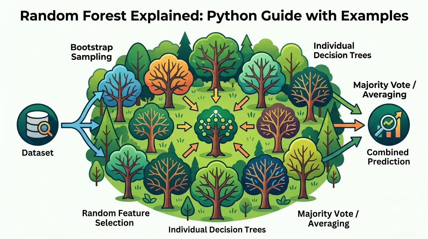
Random Forest stands as a highly popular and effective supervised machine learning algorithm. It leverages the power of ensemble learning to deliver robust and accurate predictions. This algorithm is versatile, capable of tackling both classification and regression problems with remarkable efficiency.

At its core, Random Forest combines the outputs of multiple individual Decision Trees. By doing so, it mitigates the weaknesses of single trees, leading to more stable and generalized models. This approach makes it a go-to choice for many real-world machine learning tasks.

Demystifying Random Forest: The Ensemble Learning Approach

The name "Random Forest" perfectly describes its fundamental structure: a collection, or "forest," of many individual Decision Trees. Each tree in this forest contributes to the final prediction, acting as a unique expert on a specific subset of the data.

This concept is known as ensemble learning, where multiple models are combined to achieve better predictive performance than any single model could alone. Ensemble methods harness the wisdom of crowds, averaging out individual errors and biases to produce a more reliable outcome. Random Forest is a prime example of this powerful machine learning paradigm.

Beyond Single Trees: Why Random Forest Prevents Overfitting

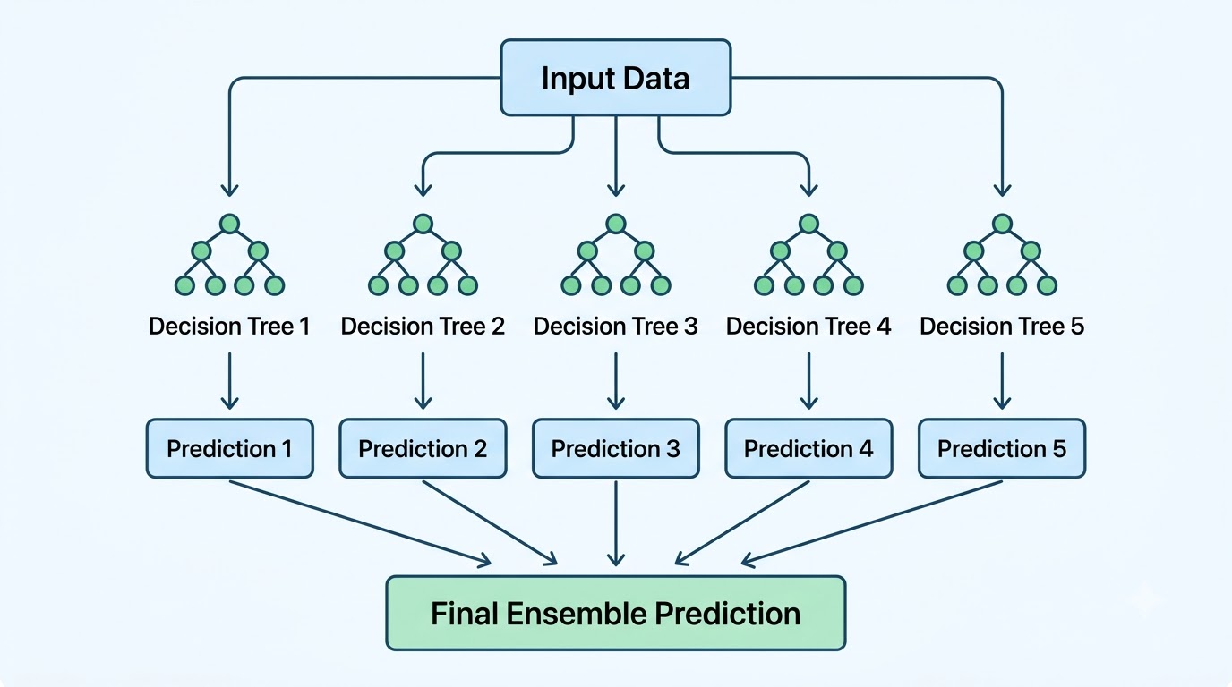
A single Decision Tree, while intuitive, often suffers from a significant drawback: its tendency to overfit the training data. This means it learns the training examples too well, including noise and outliers, leading to poor performance on new, unseen data. Such models are also highly sensitive to small changes in the training data, resulting in unstable predictions.

Random Forest elegantly addresses these issues by not relying on just one tree. Instead, it aggregates predictions from many diverse trees, effectively smoothing out individual tree errors and reducing variance. This ensemble approach leads to models that generalize much better to new data and provide more robust, stable predictions.

The Mechanics of Random Forest: A Detailed Workflow

The Random Forest algorithm follows a systematic process to build its powerful ensemble. It introduces randomness at two key stages: data sampling and feature selection. This dual randomness is crucial for creating diverse and independent trees.

Here's a step-by-step breakdown of how a Random Forest model is constructed and makes predictions:

1. Bootstrap Sampling: From the original training dataset, multiple random subsets are created with replacement. Each subset is used to train a different Decision Tree.
2. Building Individual Decision Trees: For each bootstrap sample, a Decision Tree is grown. Unlike standard Decision Trees, these trees are typically grown to their maximum depth without pruning, or with a limited maximum depth.
3. Random Feature Selection: At each node split within a tree, only a random subset of features is considered. This means the algorithm doesn't look at all available features to find the best split, further promoting diversity among the trees.
4. Aggregating Predictions: Once all trees are built, they make individual predictions on new data. For classification tasks, the final prediction is determined by a majority vote among the trees. For regression tasks, the final prediction is the average of all individual tree predictions.

Core Concepts: Bootstrap Aggregating (Bagging) and Feature Randomness

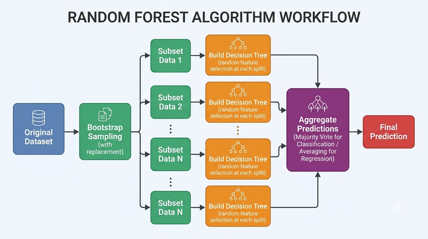
Two fundamental concepts underpin the strength and effectiveness of Random Forest: Bootstrap Aggregating, commonly known as Bagging, and random feature selection. These mechanisms are key to creating a diverse and robust ensemble of trees.

Bagging involves creating multiple subsets of the original training data by sampling with replacement. Each Decision Tree in the forest is then trained independently on one of these unique bootstrap samples. This ensures that each tree sees a slightly different version of the data, reducing correlation between trees and improving overall stability.

Beyond data sampling, Random Forest introduces another layer of randomness during the tree-building process. At each node split, instead of considering all available features, the algorithm randomly selects only a subset of features to evaluate. This forces individual trees to explore different feature combinations, preventing any single dominant feature from dictating all splits and further enhancing tree diversity.

Adapting Random Forest: Classification and Regression

Random Forest is a versatile algorithm, adept at handling both classification and regression tasks. The core principle of ensemble learning remains the same, but the method of aggregating individual tree predictions differs based on the problem type.

For classification problems, where the goal is to predict a categorical label, each Decision Tree in the forest casts a "vote" for a particular class. The final prediction of the Random Forest is then determined by the class that receives the majority of votes from all the trees. This majority voting scheme helps to smooth out individual tree errors and arrive at a more confident classification.

In regression problems, where the objective is to predict a continuous numerical value, each Decision Tree outputs its own numerical prediction. The Random Forest then combines these individual predictions by averaging them. This averaging process helps to reduce the variance of the overall model, leading to more stable and accurate continuous predictions.

Random Forest vs. Decision Tree: Choosing the Right Algorithm

While Random Forest is built upon Decision Trees, it addresses many of their inherent limitations, offering a more robust solution for most predictive tasks. Understanding their differences is crucial for selecting the appropriate algorithm for your specific problem.

A single Decision Tree is easy to interpret and visualize, making it excellent for understanding feature relationships. However, it is prone to overfitting and can be unstable, meaning small changes in data can lead to very different tree structures. Random Forest, by combining many trees, sacrifices some interpretability for significantly improved accuracy and generalization.

The ensemble nature of Random Forest makes it more computationally intensive during training compared to a single tree. However, its ability to handle complex, non-linear relationships and its inherent resistance to overfitting often make it the superior choice for high-performance applications.

Tuning Your Forest: Key Hyperparameters for Optimal Performance

To get the best performance from your Random Forest model, it's essential to understand and tune its hyperparameters. These parameters control the structure and behavior of the individual trees and the overall ensemble, influencing model complexity and diversity.

Here are some of the most important hyperparameters to consider:

1. n_estimators: This parameter defines the number of Decision Trees in the forest. A higher number generally leads to better performance but also increases computation time. It's often beneficial to increase this until performance plateaus.
2. max_depth: This controls the maximum depth of each individual tree. Limiting the depth helps prevent individual trees from overfitting, though Random Forest is already robust to this. A smaller max_depth can reduce training time.
3. max_features: This specifies the number of features to consider when looking for the best split at each node. A smaller max_features increases the diversity of the trees, which is crucial for Random Forest's effectiveness. Common values include sqrt (square root of total features) or log2.
4. min_samples_split: This is the minimum number of samples required to split an internal node. Increasing this value can prevent a tree from learning relationships that are too specific to the training data, thus reducing overfitting.
5. min_samples_leaf: This sets the minimum number of samples required to be at a leaf node. Similar to min_samples_split, a higher value ensures that splits only occur when there's a sufficient number of samples, leading to more generalized leaves.

Prerequisites: Installing Libraries for Random Forest in Python

Before diving into the practical implementation of Random Forest, you'll need to set up your Python environment. This involves installing several key libraries that provide the necessary tools for data manipulation, model building, and visualization.

The primary library for machine learning in Python is Scikit-learn, which includes the Random Forest algorithm. We'll also use Pandas for data handling, NumPy for numerical operations, and Matplotlib/Seaborn for plotting results. You can install these using pip:

pip install scikit-learn pandas numpy matplotlib seaborn

Once installed, you're ready to import these libraries into your Python scripts or Jupyter notebooks. This setup ensures you have all the tools required to build, train, and evaluate your Random Forest models effectively.

Practical Implementation: Random Forest Classification in Python

Let's put theory into practice by building a Random Forest classifier using Python and Scikit-learn. We will use the famous Iris dataset, a classic benchmark for classification tasks, to demonstrate the workflow. This dataset contains measurements of iris flowers and their corresponding species.

The process involves loading the data, splitting it into training and testing sets, initializing and training the Random Forest model, and finally making predictions. We will then evaluate the model's performance using standard classification metrics.

Loading and Inspecting the Dataset

First, we need to load the Iris dataset. Scikit-learn provides a convenient way to load this dataset directly. After loading, it's good practice to inspect the data to understand its structure and content.

import pandas as pd
from sklearn.datasets import loadᵢris

# Load the Iris dataset
iris = loadᵢris()
X = pd.DataFrame(iris.data, columns=iris.featureₙames)
y = pd.Series(iris.target)

# Display the first 5 rows of the features
print("Features (X.head()):")
print(X.head())

# Display basic information about the dataset
print("\nDataset Info (X.info()):")
X.info()

# Display descriptive statistics of the features
print("\nDescriptive Statistics (X.describe()):")
print(X.describe())

# Display the target variable unique values and counts
print("\nTarget unique values (y.value_counts()):")
print(y.value_counts())

The output shows the first few rows of the features, their data types, and summary statistics. We can see four numerical features and a target variable with three distinct classes (0, 1, 2) representing the three iris species.

Splitting Data into Training and Testing Sets

To properly evaluate our model, we must split the dataset into training and testing sets. The training set is used to teach the model, while the testing set provides an unbiased evaluation of its performance on unseen data. A common split ratio is 70% for training and 30% for testing.

from sklearn.model_selection import train_test_split

# Split the data into training and testing sets
# test_size=0.3 means 30% of the data will be used for testing
# random_state ensures reproducibility of the split
X_train, X_test, y_train, y_test = train_test_split(X, y, test_size=0.3, random_state=42)

# Print the shapes of the resulting datasets
print(f"X_train shape: {X_train.shape")
print(f"X_test shape: {X_test.shape")
print(f"y_train shape: {y_train.shape")
print(f"y_test shape: {y_test.shape")

This code snippet divides our dataset, ensuring that both feature data (X) and target labels (y) are split consistently. The random_state parameter guarantees that the split is the same every time you run the code, which is crucial for reproducible results.

Initializing and Training the Random Forest Classifier

Now, we'll import the RandomForestClassifier from Scikit-learn, instantiate it with some initial hyperparameters, and then train it using our training data. The n_estimators parameter specifies the number of trees in the forest, and random_state ensures reproducibility.

from sklearn.ensemble import RandomForestClassifier

# Initialize the Random Forest Classifier
# n_estimators=100 means 100 decision trees will be built
# random_state=42 ensures reproducibility
rf_classifier = RandomForestClassifier(n_estimators=100, random_state=42)

# Train the model using the training data
print("Training Random Forest Classifier...")
rf_classifier.fit(X_train, y_train)
print("Training complete.")

The fit() method is where the Random Forest algorithm learns patterns from the X_train features to predict the y_train labels. This process involves building all 100 individual decision trees based on bootstrap samples and random feature subsets.

Making Predictions with the Trained Model

After training, our Random Forest classifier is ready to make predictions on new, unseen data. We will use the predict() method on our X_test set to obtain the model's classifications. These predictions will then be compared against the actual y_test labels to assess performance.

# Continued from previous block - requires rf_classifier and X_test

# Make predictions on the test set
y_pred_rf_clf = rf_classifier.predict(X_test)

# Display the first few predictions and actual values for comparison
print("First 10 predictions:", y_pred_rf_clf[:10])
print("First 10 actual values:", y_test.values[:10])

The y_pred_rf_clf array now holds the predicted species for each flower in our test set. Comparing these predictions to the actual y_test values gives us an initial glimpse into the model's accuracy, which we will quantify in the next section.

Assessing Performance: Evaluating Random Forest Classification

Evaluating a classification model is crucial to understand how well it performs. For Random Forest classifiers, we use several key metrics that provide a comprehensive view of its accuracy, precision, recall, and overall F1-score. These metrics help us understand not just how many predictions are correct, but also the types of errors the model makes.

We will also visualize the confusion matrix, which offers a detailed breakdown of true positives, true negatives, false positives, and false negatives. This visual representation is invaluable for diagnosing specific performance issues.

Accuracy, Precision, Recall, and F1-Score

These metrics are fundamental for evaluating classification models. Accuracy measures the proportion of correctly classified instances. Precision focuses on the correctness of positive predictions, while Recall measures the model's ability to find all positive instances. The F1-score is the harmonic mean of precision and recall, offering a balanced measure.

from sklearn.metrics import classification_report, accuracy_score

# Continued from previous block - requires y_test and y_pred_rf_clf

# Calculate overall accuracy
accuracy = accuracy_score(y_test, y_pred_rf_clf)
print(f"Accuracy: {accuracy:.4f")

# Generate a detailed classification report
# This includes precision, recall, f1-score, and support for each class
print("\nClassification Report:")
print(classification_report(y_test, y_pred_rf_clf, targetₙames=iris.targetₙames))

The classification report provides a per-class breakdown of these metrics, which is especially useful for multi-class problems like the Iris dataset. A high accuracy and balanced precision/recall across classes indicate a well-performing model.

Understanding the Confusion Matrix

The confusion matrix is a table that summarizes the performance of a classification algorithm. Each row represents the instances in an actual class, while each column represents the instances in a predicted class. It clearly shows where the model made correct predictions and where it made errors.

import matplotlib.pyplot as plt
import seaborn as sns
from sklearn.metrics import confusion_matrix

# Continued from previous block - requires y_test and y_pred_rf_clf

# Generate the confusion matrix
cm = confusion_matrix(y_test, y_pred_rf_clf)

# Plot the confusion matrix using Seaborn
plt.figure(figsize=(8, 6))
sns.heatmap(cm, annot=True, fmt='d', cmap='Blues',
            xticklabels=iris.targetₙames, yticklabels=iris.targetₙames)
plt.title('Confusion Matrix for Random Forest Classifier')
plt.xlabel('Predicted Label')
plt.ylabel('True Label')
plt.show()

In the confusion matrix, diagonal elements represent correctly classified instances (True Positives/Negatives). Off-diagonal elements indicate misclassifications (False Positives/Negatives). A perfectly performing model would have all non-zero values only on the main diagonal.

Practical Implementation: Random Forest Regression in Python

Random Forest is equally powerful for regression tasks, where the goal is to predict a continuous numerical output. We will now demonstrate its application using a regression problem, specifically the California Housing dataset. This dataset contains median house values for districts in California.

The workflow for regression is very similar to classification: load and prepare the data, split it, train the regressor, and make predictions. The main difference lies in the choice of model (RandomForestRegressor) and the evaluation metrics.

Loading and Preparing Regression Data

We'll load the California Housing dataset, which is also available through Scikit-learn. This dataset is larger and more complex than Iris, providing a good example for regression. We'll separate the features (X) from the target variable (y), which is the median house value.

import pandas as pd
from sklearn.datasets import fetch_california_housing

# Load the California Housing dataset
housing = fetch_california_housing(as_frame=True)
X_housing = housing.data
y_housing = housing.target

# Display the first 5 rows of the features
print("Features (X_housing.head()):")
print(X_housing.head())

# Display basic information about the dataset
print("\nDataset Info (X_housing.info()):")
X_housing.info()

# Display descriptive statistics of the features
print("\nDescriptive Statistics (X_housing.describe()):")
print(X_housing.describe())

The dataset contains 8 features describing various aspects of housing districts and a target variable representing the median house value in hundreds of thousands of dollars. We can observe the scale and distribution of these features from the descriptive statistics.

Initializing and Training the Random Forest Regressor

Similar to the classifier, we import RandomForestRegressor, instantiate it, and train it on the housing data. We'll use the same train_test_split function to prepare our data for training and evaluation. The n_estimators parameter is again crucial for controlling the number of trees.

from sklearn.ensemble import RandomForestRegressor
from sklearn.model_selection import train_test_split

# Continued from previous block - requires X_housing, y_housing

# Split the data into training and testing sets for regression
X_train_reg, X_test_reg, y_train_reg, y_test_reg = train_test_split(X_housing, y_housing, test_size=0.3, random_state=42)

# Initialize the Random Forest Regressor
# n_estimators=100 means 100 decision trees will be built
# random_state=42 ensures reproducibility
rf_regressor = RandomForestRegressor(n_estimators=100, random_state=42, nⱼobs=-1)

# Train the model using the training data
print("Training Random Forest Regressor...")
rf_regressor.fit(X_train_reg, y_train_reg)
print("Training complete.")

The nⱼobs=-1 parameter allows the model to use all available CPU cores for training, significantly speeding up the process for larger datasets. The fit() method builds the ensemble of decision trees, each learning to predict median house values.

Making Predictions

With the Random Forest Regressor trained, we can now use it to make predictions on the test set. The predict() method will output continuous numerical values, representing the model's estimated median house prices for each district in X_test_reg.

# Continued from previous block - requires rf_regressor and X_test_reg

# Make predictions on the test set
y_pred_rf_reg = rf_regressor.predict(X_test_reg)

# Display the first few predictions and actual values for comparison
print("First 10 predictions:", y_pred_rf_reg[:10])
print("First 10 actual values:", y_test_reg.values[:10])

These predictions represent the model's best guess for the median house values. We will compare these predicted values against the actual y_test_reg values in the next section to quantify the model's accuracy using specific regression metrics.

Assessing Performance: Evaluating Random Forest Regression

Evaluating regression models requires different metrics than classification models, as we are dealing with continuous outputs. Key metrics help us understand the magnitude of errors and how well the model's predictions align with actual values.

We will focus on Mean Absolute Error (MAE), Mean Squared Error (MSE), Root Mean Squared Error (RMSE), and R-squared (R²). These metrics provide a comprehensive view of the model's predictive accuracy and explanatory power.

Mean Absolute Error (MAE) and Mean Squared Error (MSE)

MAE measures the average magnitude of the errors in a set of predictions, without considering their direction. It's robust to outliers. MSE, on the other hand, measures the average of the squares of the errors, giving more weight to larger errors. Both are commonly used to quantify prediction accuracy.

from sklearn.metrics import mean_absolute_error, mean_squared_error

# Continued from previous block - requires y_test_reg and y_pred_rf_reg

# Calculate Mean Absolute Error (MAE)
mae = mean_absolute_error(y_test_reg, y_pred_rf_reg)
print(f"Mean Absolute Error (MAE): {mae:.4f")

# Calculate Mean Squared Error (MSE)
mse = mean_squared_error(y_test_reg, y_pred_rf_reg)
print(f"Mean Squared Error (MSE): {mse:.4f")

A lower MAE indicates that the model's predictions are, on average, closer to the actual values. A lower MSE also signifies better performance, but its squared nature means it penalizes larger errors more heavily, making it sensitive to outliers.

Root Mean Squared Error (RMSE) and R-squared (R²)

RMSE is the square root of MSE, bringing the error metric back to the same units as the target variable, making it more interpretable. R-squared, or the coefficient of determination, measures the proportion of the variance in the dependent variable that is predictable from the independent variables. It indicates how well the model explains the variability of the target variable.

import numpy as np
from sklearn.metrics import r2_score

# Continued from previous block - requires y_test_reg, y_pred_rf_reg, and mse

# Calculate Root Mean Squared Error (RMSE)
rmse = np.sqrt(mse)
print(f"Root Mean Squared Error (RMSE): {rmse:.4f")

# Calculate R-squared (R²)
r2 = r2_score(y_test_reg, y_pred_rf_reg)
print(f"R-squared (R²): {r2:.4f")

A higher R-squared value (closer to 1) indicates that the model explains a larger proportion of the variance in the target variable, suggesting a better fit. RMSE provides an interpretable error magnitude, directly comparable to the scale of the target variable.

Unveiling Insights: Feature Importance with Random Forest

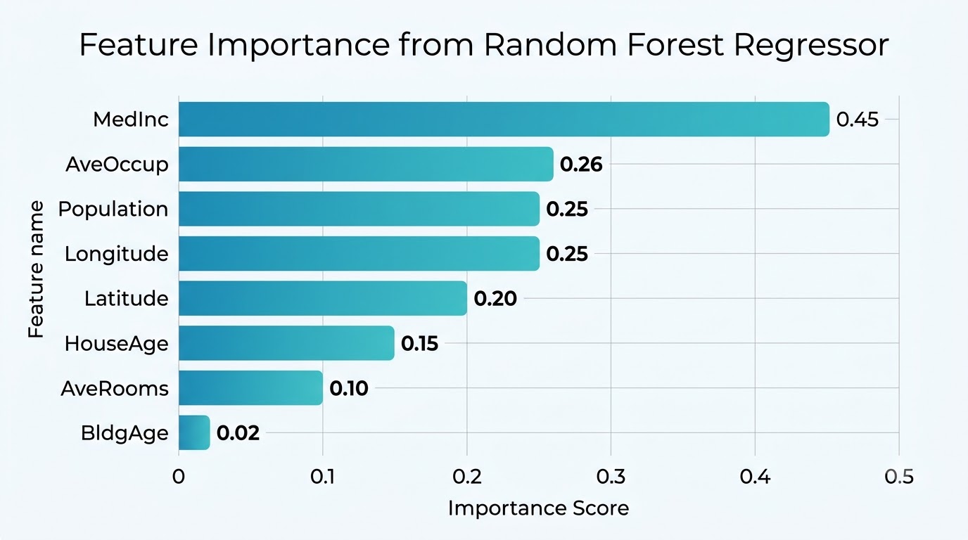
One of the significant advantages of Random Forest is its ability to inherently provide feature importance scores. These scores quantify the contribution of each feature to the model's predictive power. This insight is invaluable for understanding which factors are most influential in determining the target variable.

Feature importance is calculated by measuring how much each feature reduces impurity (e.g., Gini impurity for classification, MSE for regression) across all trees in the forest. Features that consistently lead to significant impurity reduction are deemed more important. This allows developers to interpret the model and potentially perform feature selection.

import matplotlib.pyplot as plt
import numpy as np

# Continued from previous block - requires rf_regressor and X_housing

# Get feature importances from the trained regressor
featureᵢmportances = rf_regressor.featureᵢmportances_

# Get feature names from the dataset
featureₙames = X_housing.columns

# Create a pandas Series for easier sorting and plotting
importance_df = pd.Series(featureᵢmportances, index=featureₙames).sort_values(ascending=False)

# Print feature importances
print("\nFeature Importances (Top 10):\n", importance_df.head(10))

# Plot feature importances
plt.figure(figsize=(10, 6))
sns.barplot(x=importance_df.values, y=importance_df.index, palette='viridis')
plt.title('Feature Importance from Random Forest Regressor')
plt.xlabel('Importance Score')
plt.ylabel('Feature Name')
plt.tight_layout()
plt.show()

The bar plot visually represents the relative importance of each feature. Features with higher bars contribute more significantly to the model's predictions. This information can guide further data collection, feature engineering, or even simplify the model by removing less important features.

Optimizing Your Random Forest: Best Practices and Avoiding Pitfalls

While Random Forest is robust, applying best practices can significantly enhance its performance and reliability. Proper hyperparameter tuning, careful handling of data imbalances, and robust validation techniques are crucial for building effective models.

Here are some key considerations for optimizing your Random Forest models:

1. Hyperparameter Tuning: Use techniques like GridSearchCV or RandomizedSearchCV from Scikit-learn to systematically search for the best combination of hyperparameters. This automates the process of finding optimal n_estimators, max_depth, max_features, etc.
2. Cross-Validation: Always use cross-validation (e.g., K-Fold cross-validation) to get a more reliable estimate of your model's performance. This helps ensure your model generalizes well to unseen data and isn't just performing well on a single train-test split.
3. Handling Imbalanced Datasets: For classification tasks with imbalanced classes, standard Random Forest might favor the majority class. Techniques like class_weight parameter, SMOTE (Synthetic Minority Over-sampling Technique), or RandomForestClassifier with balanced or balanced_subsample options can help.
4. Feature Engineering: While Random Forest handles many features well, thoughtful feature engineering can still provide significant boosts. Creating new, more informative features from existing ones can help the trees find better splits.

Avoid common pitfalls such as using an excessively large number of trees (n_estimators) without performance gain, which only increases computation time. While Random Forest is less sensitive to feature scaling, it's still good practice to understand your data's scale. Lastly, remember that feature importance indicates statistical relevance, not necessarily causal relationships.

Random Forest in Action: Pros, Cons, and Use Cases

Random Forest is a highly versatile and powerful algorithm, widely adopted across various industries due to its robust performance. However, like any machine learning model, it comes with its own set of advantages and limitations that are important to consider.

Advantages of Random Forest

1. Reduced Overfitting: By averaging multiple deep decision trees, Random Forest significantly reduces the risk of overfitting, leading to better generalization on unseen data.
2. High Accuracy: It often achieves high accuracy compared to single decision trees and many other algorithms, especially on complex datasets.
3. Handles Non-Linearity: Random Forest can naturally model non-linear relationships between features and the target variable without requiring explicit transformations.
4. Works with Many Features: It performs well even with a large number of features, including redundant ones, due to its random feature selection mechanism.
5. Implicit Feature Selection: The algorithm provides built-in feature importance scores, helping identify the most influential features in the dataset.
6. Handles Missing Values (with imputation): While Scikit-learn requires pre-imputation, the tree structure is robust to various imputation strategies.

Limitations of Random Forest

1. Higher Computational Cost: Training many trees can be computationally expensive and time-consuming, especially with a large number of n_estimators and a vast dataset.
2. Reduced Interpretability: The ensemble nature makes it a "black box" model. It's harder to visualize and interpret the decision-making process compared to a single decision tree.
3. Memory Intensive: Storing many decision trees can consume a significant amount of memory, particularly for large forests.

Real-World Use Cases

Random Forest's versatility makes it suitable for a wide array of applications across various industries:

1. Fraud Detection: Identifying fraudulent transactions in banking and finance by classifying suspicious activities.
2. Medical Diagnosis: Predicting disease outcomes, classifying tumors (benign/malignant), and identifying risk factors based on patient data.
3. Stock Market Prediction: Forecasting stock prices or market trends, though this is a highly complex and challenging domain.
4. Customer Churn Prediction: Predicting which customers are likely to leave a service, allowing companies to implement retention strategies.
5. Image Classification: Used in computer vision for tasks like object recognition and image segmentation, often as part of larger pipelines.
6. E-commerce: Recommending products to users, predicting product demand, and segmenting customers based on purchasing behavior.

Conclusion: Harnessing the Ensemble Power of Random Forest

Random Forest is a cornerstone algorithm in machine learning, celebrated for its ability to deliver high accuracy and robustness. By intelligently combining the predictions of numerous diverse decision trees, it effectively mitigates the common pitfalls of individual models, particularly overfitting.

Its dual mechanisms of bootstrap aggregating and random feature selection ensure that each tree contributes uniquely to the ensemble, leading to stable and generalized predictions for both classification and regression tasks. The inherent feature importance scores also provide valuable insights into your data.

As you continue your machine learning journey, consider exploring other advanced ensemble methods. Algorithms like Gradient Boosting, XGBoost, and LightGBM build upon similar principles but offer different approaches to combining models, often achieving even higher performance in competitive scenarios. Mastering Random Forest is an excellent foundation for delving into these powerful techniques.