Linear Regression Explained with Python Code and Examples

Introduction to Linear Regression: The Foundation of Predictive Analytics

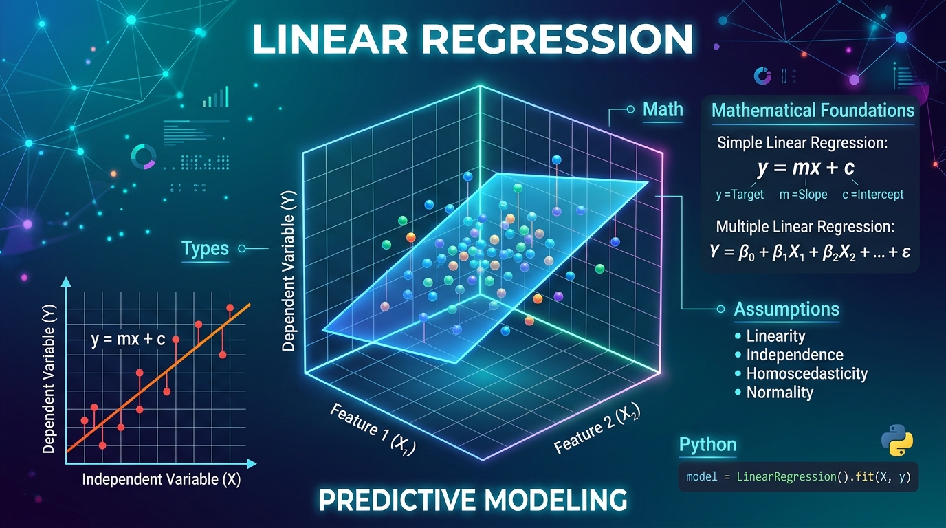
Linear Regression stands as a cornerstone in the world of machine learning and statistics. It is a fundamental supervised learning algorithm, widely recognized for its simplicity and interpretability. This algorithm forms the bedrock for understanding more complex predictive models.

For both beginners and seasoned data scientists, mastering Linear Regression is crucial. It provides essential insights into relationships between variables and serves as a powerful tool for making predictions. Its widespread use spans across numerous industries, tackling diverse real-world prediction challenges.

What Exactly is Linear Regression?

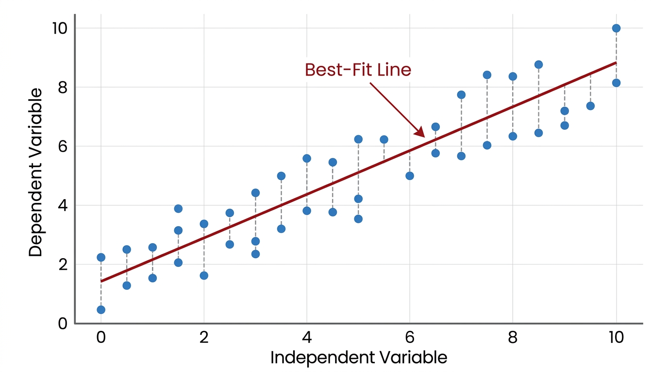
Linear Regression is a statistical method used to model the relationship between a dependent variable and one or more independent variables. Its primary goal is to predict a continuous outcome. Think of it as drawing a straight line through a set of data points.

This 'best-fit line' (or hyperplane in higher dimensions) represents the average relationship between the variables. For instance, imagine predicting a student's exam score based on their study hours. Linear Regression helps find the line that best describes how study hours influence scores.

Types of Linear Regression: Simple vs. Multiple

Linear Regression primarily comes in two forms, distinguished by the number of independent variables they utilize. Understanding these types is key to applying the correct model for your data. Each type addresses different complexities in variable relationships.

Simple Linear Regression involves one independent variable, making it straightforward for analyzing direct relationships. Multiple Linear Regression, conversely, uses two or more independent variables, allowing for more nuanced and comprehensive predictive modeling.

Mathematical Intuition Behind Linear Regression

At its core, Linear Regression is built upon a simple linear equation. For Simple Linear Regression, this is often expressed as y = mx + c, where 'y' is the dependent variable, 'x' is the independent variable, 'm' is the slope, and 'c' is the y-intercept. In machine learning, 'm' is often called the coefficient (β₁) and 'c' the intercept (β₀).

For Multiple Linear Regression, the equation expands to Y = β₀ + β₁X1 + β₂X2 + ... + βₙXn. Here, β₀ is the intercept, and β₁, β₂, ..., βₙ are the coefficients for each independent variable X1, X2, ..., Xn. These coefficients represent the change in Y for a one-unit change in the corresponding X, assuming all other X variables remain constant.

The model's goal is to find the values for these coefficients (β₀, β₁, etc.) that minimize the difference between the predicted values and the actual values. These differences are known as residuals or errors. Minimizing these errors ensures the 'best-fit' line accurately represents the data's trend.

The Cost Function: Quantifying and Minimizing Prediction Error

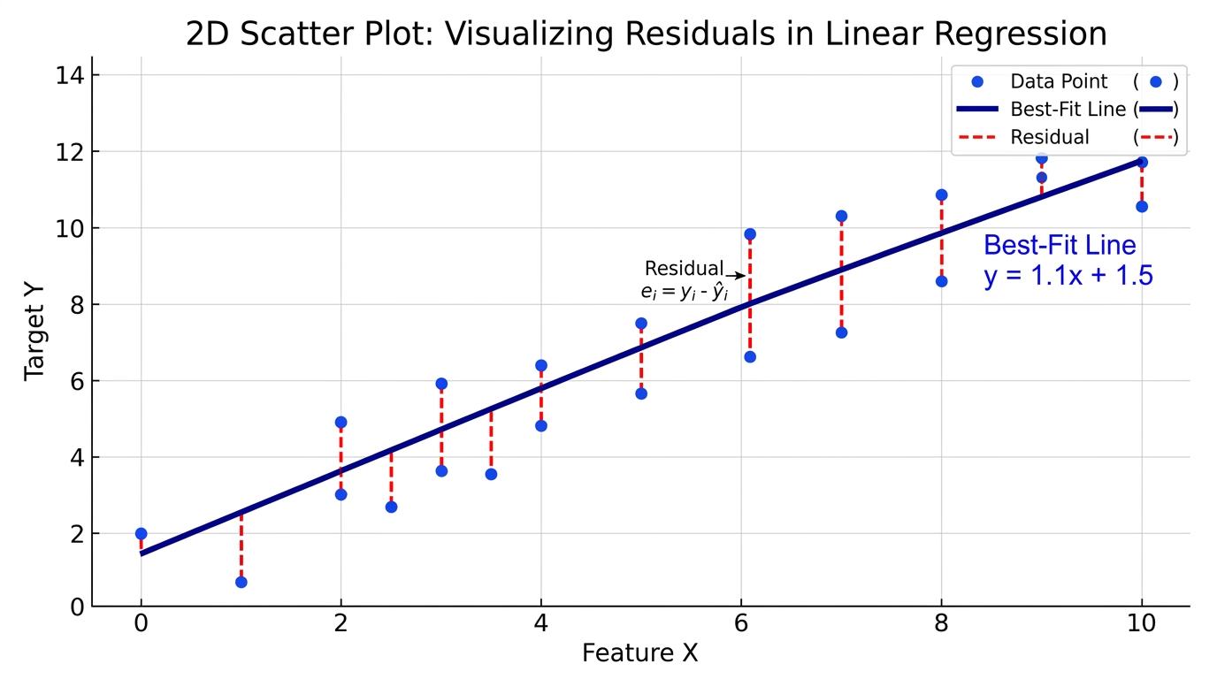
To find the optimal coefficients, Linear Regression uses a cost function, often the Mean Squared Error (MSE). The cost function quantifies the overall difference between the predicted values and the actual observed values. It essentially measures how 'wrong' our model's predictions are.

The objective is to minimize this cost function. By minimizing MSE, the algorithm finds the set of coefficients that results in the smallest average squared error. This process leads to the most accurate 'best-fit' line for the given data. The MSE function is convex, meaning it has a single global minimum, which simplifies the optimization process.

Gradient Descent: The Algorithm for Optimization

Gradient Descent is an iterative optimization algorithm used to minimize the cost function. It works by repeatedly adjusting the model's parameters (coefficients and intercept) in the direction that reduces the cost. Imagine rolling a ball down a hill; Gradient Descent finds the steepest path downwards to reach the valley floor, which represents the minimum cost.

Each step in Gradient Descent involves calculating the gradient (slope) of the cost function with respect to each parameter. The parameters are then updated by subtracting a fraction of this gradient, determined by the 'learning rate'. The learning rate is a crucial hyperparameter that controls the size of these steps; a small learning rate can make convergence slow, while a large one might cause overshooting the minimum.

Key Assumptions of Linear Regression and Their Importance

Linear Regression models rely on several critical assumptions for their results to be valid and interpretable. Violating these assumptions can lead to unreliable coefficients, inaccurate predictions, and misleading statistical inferences. It's essential to check these assumptions before trusting your model.

Understanding these assumptions helps in diagnosing model issues and choosing appropriate remedies. They guide data preprocessing and feature engineering decisions. Let's explore each assumption in detail.

1. Linearity: The Relationship Between Variables

The first assumption is that a linear relationship exists between the independent variables and the dependent variable. This means the change in the dependent variable due to a one-unit change in an independent variable is constant. If the relationship is non-linear, a linear model will fail to capture the true underlying pattern.

You can check for linearity using scatter plots between each independent variable and the dependent variable. If non-linearity is detected, consider data transformations (e.g., logarithmic, square root) or using polynomial regression to model the curved relationship.

2. Independence of Residuals: No Autocorrelation

This assumption states that the residuals (errors) should be independent of each other. In simpler terms, the error for one observation should not be correlated with the error for another observation. This is particularly crucial in time-series data, where consecutive observations often exhibit dependence.

Violations, known as autocorrelation, can lead to underestimated standard errors and inflated R²-squared values. The Durbin-Watson test is a common statistical test used to detect the presence of autocorrelation in residuals. Addressing autocorrelation often involves using time-series specific models or including lagged variables.

3. Homoscedasticity: Constant Variance of Residuals

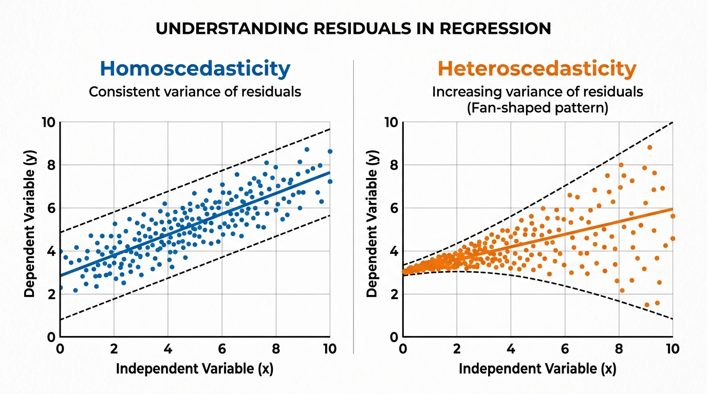
Homoscedasticity means that the variance of the residuals is constant across all levels of the independent variables. In other words, the spread of the errors should be roughly the same regardless of the predicted value. The opposite, heteroscedasticity, occurs when the error variance changes with the independent variables.

Heteroscedasticity can lead to inefficient coefficient estimates and incorrect standard errors, affecting hypothesis tests. Residual plots (plotting residuals against predicted values) are excellent for checking this assumption; a random scatter indicates homoscedasticity, while a funnel shape suggests heteroscedasticity. Transformations of the dependent variable or weighted least squares regression can help mitigate this issue.

4. Normality of Residuals: Bell-Shaped Distribution

The assumption of normality states that the residuals should be approximately normally distributed. While not strictly required for coefficient estimation, it is important for valid hypothesis testing, confidence intervals, and p-value interpretations. If residuals are not normal, statistical inferences about the coefficients might be unreliable.

You can check for normality using Q-Q plots, histograms of residuals, or statistical tests like the Shapiro-Wilk test. If residuals deviate significantly from normality, transformations of the dependent variable or using robust regression methods might be considered. However, for large sample sizes, the Central Limit Theorem often ensures that coefficient estimates are approximately normal even if residuals are not.

5. No Multicollinearity: Independent Predictors

Multicollinearity occurs when two or more independent variables in a multiple regression model are highly correlated with each other. While it doesn't affect the model's predictive power, it can severely impact the interpretability of individual coefficients. High multicollinearity makes it difficult to determine the individual effect of each predictor on the dependent variable.

It can also lead to unstable and highly sensitive coefficient estimates, where small changes in the data result in large changes in coefficients. The Variance Inflation Factor (VIF) is a common metric to detect multicollinearity; VIF values above 5 or 10 typically indicate a problem. Strategies to mitigate multicollinearity include removing one of the correlated variables, combining them, or using dimensionality reduction techniques like Principal Component Analysis (PCA).

How Linear Regression Works: A Step-by-Step Process

Building a Linear Regression model involves a systematic workflow, from preparing your data to evaluating the model's performance. Each step is crucial for developing a robust and accurate predictive tool. Let's outline the typical process.

This structured approach ensures that the model is trained effectively and its predictions are reliable. It also provides opportunities to diagnose and address potential issues at various stages.

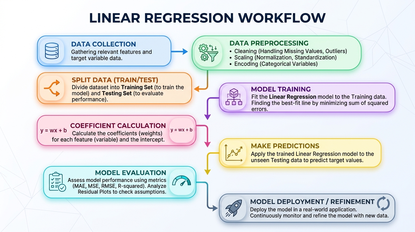
Here's a breakdown of the key steps:

1. Data Preparation: This involves collecting relevant data, cleaning it by handling missing values and outliers, and transforming features if necessary (e.g., scaling numerical features, encoding categorical ones). The quality of your data directly impacts model performance.
2. Splitting Data: The dataset is divided into training and testing sets. The training set is used to teach the model, while the testing set evaluates its performance on unseen data, ensuring unbiased assessment.
3. Model Training: The Linear Regression algorithm is applied to the training data. During this phase, the model learns the optimal coefficients and intercept that minimize the cost function, typically using Ordinary Least Squares (OLS) or Gradient Descent.
4. Coefficient Calculation: Once trained, the model provides the calculated coefficients for each independent variable and the intercept. These values define the 'best-fit' line or hyperplane.
5. Prediction Generation: The trained model is then used to make predictions on the independent variables from the test set. These predictions are the model's estimated output values.
6. Model Evaluation: Finally, the predicted values are compared against the actual values from the test set. Various metrics are used to quantify the model's accuracy and performance, helping to understand how well it generalizes to new data.

Evaluating Your Linear Regression Model: Key Metrics

After training a Linear Regression model, it's crucial to evaluate its performance to understand how well it makes predictions. Several metrics are commonly used for this purpose, each offering a different perspective on the model's accuracy and error. Choosing the right metric depends on the specific problem and business context.

These metrics help in comparing different models, fine-tuning hyperparameters, and ensuring the model meets performance expectations. Let's delve into the most important ones.

Mean Absolute Error (MAE)

Mean Absolute Error (MAE) is the average of the absolute differences between the predicted values and the actual values. It provides a straightforward measure of the average magnitude of errors. MAE is expressed in the same units as the dependent variable, making it highly interpretable.

One of MAE's key advantages is its robustness to outliers. Since it takes the absolute difference, extreme errors do not disproportionately influence the overall error metric, unlike squared error metrics. This makes it a good choice when you want a balanced view of error without heavily penalizing large deviations.

Mean Squared Error (MSE) and Root Mean Squared Error (RMSE)

Mean Squared Error (MSE) calculates the average of the squared differences between predicted and actual values. By squaring the errors, MSE heavily penalizes larger errors, making it sensitive to outliers. This characteristic is useful when large prediction errors are particularly undesirable or costly.

Root Mean Squared Error (RMSE) is simply the square root of MSE. Taking the square root brings the error metric back into the same units as the dependent variable, which improves interpretability compared to MSE. RMSE is one of the most widely used metrics for regression tasks due to its balance of penalizing large errors and being in interpretable units.

R²-squared (R²) Score and Adjusted R²

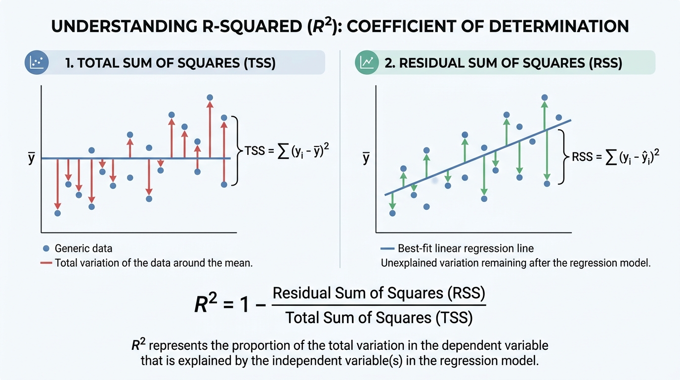
The R²-squared (R²) score, also known as the coefficient of determination, measures the proportion of the variance in the dependent variable that is predictable from the independent variables. It ranges from 0 to 1, where 1 indicates that the model perfectly explains the variance of the target variable. An R² of 0.75 means that 75% of the variation in the dependent variable can be explained by the model.

While R² is a good 'goodness of fit' measure, it has a limitation: it tends to increase as you add more independent variables to the model, even if those variables are not truly predictive. Adjusted R² addresses this by penalizing the addition of unnecessary predictors. It provides a more reliable measure for multiple linear regression, especially when comparing models with different numbers of features, as it only increases if the new predictor improves the model more than would be expected by chance.

Advantages and Limitations of Linear Regression

Linear Regression, despite its simplicity, offers significant advantages that make it a popular choice for many predictive tasks. Its interpretability is a major strength, allowing stakeholders to easily understand the impact of each feature. The model's coefficients directly show the magnitude and direction of influence.

Furthermore, Linear Regression is computationally efficient and easy to implement, even on large datasets. It provides a solid baseline for more complex models and performs exceptionally well when the relationship between variables is truly linear. Its straightforward nature makes it an excellent starting point for any predictive analytics project.

However, Linear Regression also comes with notable limitations. It assumes a linear relationship, meaning it struggles to capture complex, non-linear patterns in data. Its performance can be severely affected by outliers, as the least squares method tries to minimize the squared errors, giving disproportionate weight to extreme values.

The model's reliance on several strict assumptions (linearity, independence, homoscedasticity, normality, no multicollinearity) can also be a drawback. If these assumptions are violated, the model's results may be unreliable or misleading. In scenarios with high non-linearity, many features, or significant outliers, other machine learning algorithms might offer superior performance.

Real-World Applications of Linear Regression

Linear Regression is not just a theoretical concept; it's a workhorse in various industries, providing valuable insights and predictions. Its versatility allows it to address a wide array of business and scientific problems. Here are some concrete examples of its practical utility.

From economics to healthcare, the ability to model and predict continuous outcomes makes Linear Regression an indispensable tool. It helps in making informed decisions and understanding underlying trends.

1. House Price Prediction: Real estate companies use Linear Regression to estimate house prices based on features like size, number of bedrooms, location, and age. This helps buyers and sellers make informed decisions.
2. Salary Estimation: HR² departments and recruiters can predict an employee's salary based on years of experience, education level, role, and industry. This aids in fair compensation and budgeting.
3. Sales Forecasting: Businesses predict future sales volumes based on advertising spend, seasonality, economic indicators, and promotional activities. Accurate forecasts help in inventory management and strategic planning.
4. Demand Prediction: Retailers and logistics companies forecast product demand to optimize supply chains and prevent stockouts or overstocking. Factors like historical sales, promotions, and external events are considered.
5. Financial Forecasting: Analysts use Linear Regression to predict stock prices, commodity prices, or other financial metrics based on historical data, market trends, and economic indicators. This supports investment decisions.

Python Implementation: Building a Linear Regression Model with Scikit-learn

Let's put theory into practice by building a Linear Regression model using Python and the popular Scikit-learn library. We'll walk through each step, from setting up the environment to evaluating the model. This hands-on example will solidify your understanding.

For this demonstration, we'll use a synthetic dataset generated by Scikit-learn, which simplifies the data loading and preprocessing steps. This allows us to focus purely on the Linear Regression workflow.

Setting Up Your Environment and Importing Libraries

First, ensure you have the necessary libraries installed. If not, you can install them using pip. We'll then import these libraries, which are essential for data manipulation, modeling, and visualization.

pip install numpy pandas scikit-learn matplotlib seaborn

# Import necessary libraries
import numpy as np
import pandas as pd
import matplotlib.pyplot as plt
import seaborn as sns
from sklearn.model_selection import train_test_split
from sklearn.linear_model import LinearRegression
from sklearn.metrics import mean_absolute_error, mean_squared_error, r2_score
from sklearn.preprocessing import StandardScaler
from sklearn.datasets import make_regression # For generating a synthetic dataset

Loading and Exploring the Dataset

We'll generate a synthetic dataset using make_regression for simplicity. This function allows us to control the number of samples, features, and noise. After generation, we'll convert it into a Pandas DataFrame for easier manipulation and perform basic exploration.

# Continued from previous block -- requires the setup above

# Generate a synthetic dataset
X, y = make_regression(n_samples=1000, n_features=5, n_informative=3, noise=20, random_state=42)

# Convert to pandas DataFrame for easier handling
df = pd.DataFrame(X, columns=[f'feature_{i+1}' for i in range(X.shape[1])])
df['target'] = y

# Display the first few rows of the dataset
print("Dataset Head:")
print(df.head())

# Get basic information about the dataset
print("\nDataset Info:")
df.info()

# Get descriptive statistics
print("\nDataset Description:")
print(df.describe())

# Visualize relationships between features and target (for a few features)
# Using seaborn's pairplot can be heavy for many features, so we'll plot a few informative ones
plt.figure(figsize=(15, 5))
for i in range(3):
    plt.subplot(1, 3, i + 1)
    sns.scatterplot(x=df[f'feature_{i+1}'], y=df['target'])
    plt.title(f'Feature {i+1} vs Target')
plt.tight_layout()
plt.show()

Data Preprocessing and Feature Engineering

For our synthetic dataset, missing values and categorical variables are not an issue. However, feature scaling is often beneficial for gradient descent-based optimization algorithms. It helps them converge faster and perform better.

We'll use StandardScaler to standardize our features, transforming them to have a mean of 0 and a standard deviation of 1. This ensures that no single feature dominates the learning process due to its scale.

# Continued from previous block -- requires the setup above

# Separate features (X) and target (y)
X = df.drop('target', axis=1)
y = df['target']

# Initialize StandardScaler
scaler = StandardScaler()

# Fit the scaler on the features and transform them
X_scaled = scaler.fit_transform(X)

# Convert scaled features back to DataFrame for better readability (optional)
X_scaled_df = pd.DataFrame(X_scaled, columns=X.columns)

print("\nScaled Features Head:")
print(X_scaled_df.head())

Splitting Data into Training and Testing Sets

To evaluate our model's performance objectively, we must split our data into training and testing sets. The training set is used to train the model, while the test set simulates unseen data. This split helps us assess how well the model generalizes.

We'll use train_test_split from Scikit-learn, typically allocating 70-80% of the data for training and the remainder for testing. Setting random_state ensures reproducibility of the split.

# Continued from previous block -- requires the setup above

# Split the scaled data into training and testing sets
# test_size=0.2 means 20% of the data will be used for testing
# random_state for reproducibility
X_train, X_test, y_train, y_test = train_test_split(X_scaled, y, test_size=0.2, random_state=42)

print(f"\nTraining features shape: {X_train.shape}")
print(f"Testing features shape: {X_test.shape}")
print(f"Training target shape: {y_train.shape}")
print(f"Testing target shape: {y_test.shape}")

Training the Linear Regression Model

Now, we'll instantiate our LinearRegression model and train it using the training data. The fit method is where the model learns the relationships between features and the target variable. It calculates the optimal coefficients and intercept.

After training, we can inspect the learned coefficients and the intercept. These values define our regression equation and show the estimated impact of each feature on the target.

# Continued from previous block -- requires the setup above

# Initialize the Linear Regression model
model = LinearRegression()

# Train the model on the training data
model.fit(X_train, y_train)

# Display the learned coefficients and intercept
print("\nModel Coefficients:")
for i, col in enumerate(X.columns):
    print(f"  {col}: {model.coef_[i]:.4f}")
print(f"Model Intercept: {model.intercept_:.4f}")

Making Predictions on the Test Set

With our model trained, the next step is to use it to make predictions on the unseen test data. This allows us to assess how well the model generalizes to new, real-world scenarios. The predict method generates these estimated output values.

These predictions will then be compared against the actual y_test values to evaluate the model's accuracy. This step is crucial for understanding the model's practical utility.

# Continued from previous block -- requires the setup above

# Make predictions on the test set
y_pred = model.predict(X_test)

print("\nFirst 5 Actual vs Predicted values:")
for actual, predicted in list(zip(y_test[:5], y_pred[:5])):
    print(f"  Actual: {actual:.2f}, Predicted: {predicted:.2f}")

Evaluating Model Performance

Now we evaluate the model's performance using the metrics discussed earlier: MAE, MSE, RMSE, and R²-squared. These metrics provide quantitative measures of how well our predictions align with the actual values. They help us understand the model's accuracy and reliability.

Interpreting these scores is vital for determining if the model is fit for purpose. Lower MAE, MSE, and RMSE values indicate better performance, while a higher R²-squared value suggests a better fit to the data.

# Continued from previous block -- requires the setup above

# Calculate evaluation metrics
mae = mean_absolute_error(y_test, y_pred)
mse = mean_squared_error(y_test, y_pred)
rmse = np.sqrt(mse)
r2 = r2_score(y_test, y_pred)

print("\nModel Evaluation Metrics:")
print(f"  Mean Absolute Error (MAE): {mae:.2f}")
print(f"  Mean Squared Error (MSE): {mse:.2f}")
print(f"  Root Mean Squared Error (RMSE): {rmse:.2f}")
print(f"  R²-squared (R²) Score: {r2:.2f}")

# Interpretation of results
print("\nInterpretation:")
print(f"- MAE of {mae:.2f} means, on average, our predictions are off by {mae:.2f} units.")
print(f"- RMSE of {rmse:.2f} indicates the typical magnitude of prediction errors in the target units.")
print(f"- R²-squared of {r2:.2f} means {r2*100:.0f}% of the variance in the target variable can be explained by our model.")

Visualizing the Best-Fit Line and Residuals

Visualizing the model's performance provides intuitive insights into its fit and error distribution. For multiple linear regression, we can plot predicted values against actual values. A perfect model would show all points lying on a 45-degree line.

Additionally, plotting residuals helps us check the homoscedasticity and normality assumptions. A random scatter of residuals around zero indicates a good fit and adherence to assumptions. Any discernible pattern suggests potential issues.

# Continued from previous block -- requires the setup above

# Plotting Predicted vs Actual Values
plt.figure(figsize=(12, 6))
plt.subplot(1, 2, 1)
sns.scatterplot(x=y_test, y=y_pred)
plt.plot([y_test.min(), y_test.max()], [y_test.min(), y_test.max()], 'r--', lw=2) # 45-degree line
plt.xlabel("Actual Values")
plt.ylabel("Predicted Values")
plt.title("Actual vs Predicted Values")

# Plotting Residuals
residuals = y_test - y_pred
plt.subplot(1, 2, 2)
sns.scatterplot(x=y_pred, y=residuals)
plt.axhline(y=0, color='r', linestyle='--', lw=2)
plt.xlabel("Predicted Values")
plt.ylabel("Residuals")
plt.title("Residuals Plot")
plt.tight_layout()
plt.show()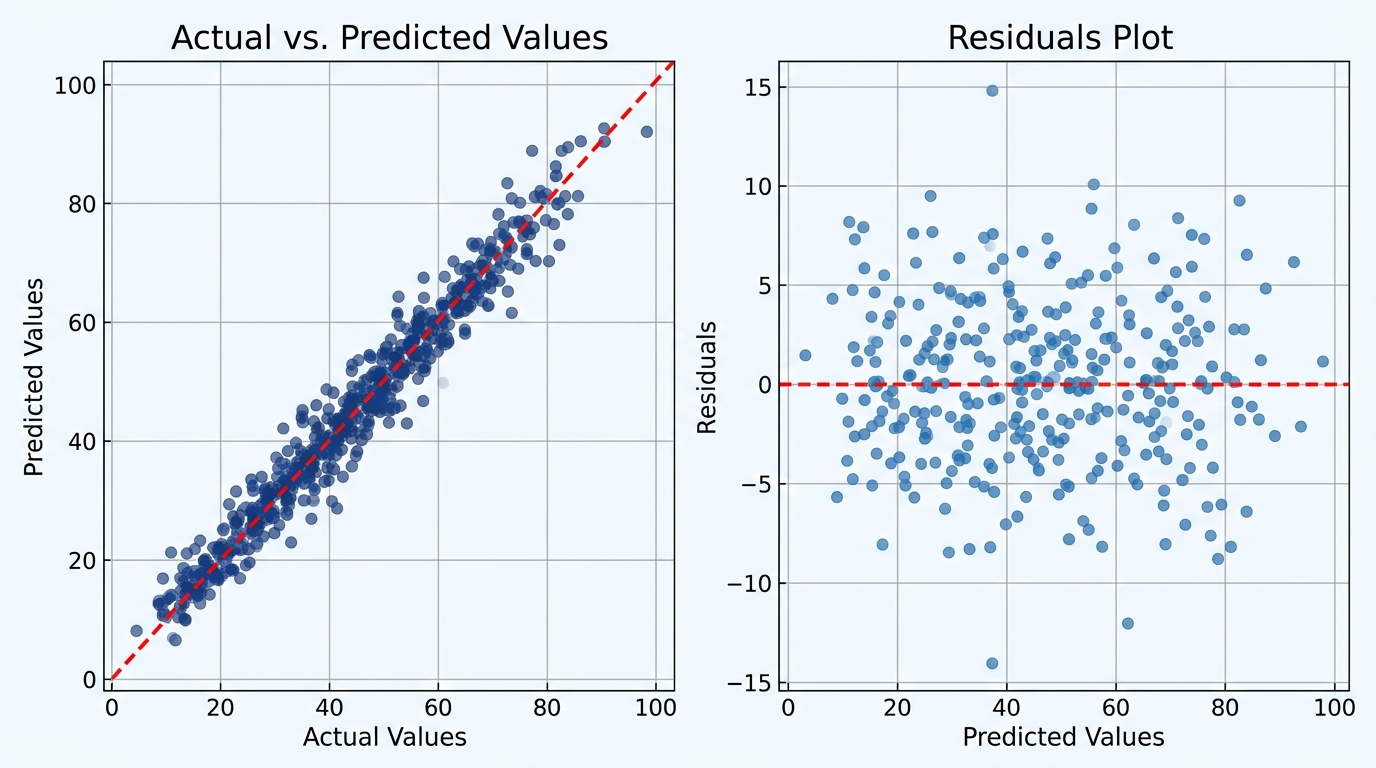

Common Mistakes to Avoid in Linear Regression

While Linear Regression is straightforward, certain pitfalls can lead to suboptimal models or incorrect interpretations. Being aware of these common mistakes can save you significant time and effort. Avoiding them ensures more reliable and robust results.

Understanding these errors helps in building better models and making more accurate predictions. Let's explore some frequent issues and how to circumvent them.

Overfitting and Underfitting

Linear Regression can suffer from both overfitting and underfitting. Underfitting occurs when the model is too simple to capture the underlying patterns in the data, leading to high bias and poor performance on both training and test sets. This often happens when important features are missing or the relationship is non-linear but a linear model is used.

Overfitting, though less common for simple linear models, can happen if too many irrelevant features are included, especially with small datasets. The model becomes too complex, capturing noise in the training data and performing poorly on unseen data. Cross-validation and regularization techniques can help diagnose and mitigate these issues.

Ignoring Multicollinearity

Ignoring multicollinearity is a common mistake that can severely impact the interpretability of your model. When independent variables are highly correlated, it becomes difficult to isolate the individual effect of each predictor on the dependent variable. This leads to unstable and unreliable coefficient estimates.

Even if the overall model's predictive power remains high, the individual coefficients might fluctuate wildly with minor changes in data. Always check for multicollinearity using VIF scores and consider feature selection or combining correlated features if necessary.

Handling Outliers Incorrectly

Outliers, which are data points significantly different from others, can heavily influence the best-fit line in Linear Regression. Since the model minimizes squared errors, a single outlier can pull the regression line towards itself, distorting the coefficients and leading to inaccurate predictions for the majority of the data. Incorrectly handling them can lead to a biased model.

It's crucial to detect outliers through visualization (e.g., box plots, scatter plots) and statistical methods. Strategies include removing them (if they are data entry errors), transforming the data (e.g., logarithmic transformation), or using robust regression techniques that are less sensitive to extreme values.

Misconceptions About Feature Scaling

A common misconception is that feature scaling (like standardization or normalization) is always strictly required for Linear Regression. For models solved using Ordinary Least Squares (OLS) with a direct mathematical solution, scaling does not affect the final coefficients or predictions. However, it does affect the magnitude of the coefficients, making them comparable.

Where scaling becomes critical is when the Linear Regression model is optimized using Gradient Descent or when regularization techniques (Ridge, Lasso) are applied. In these cases, unscaled features can lead to slow convergence or features with larger scales dominating the regularization penalty. Always scale your features if using Gradient Descent or regularization.

Incorrect Interpretation of Coefficients

Interpreting regression coefficients incorrectly is a frequent error. A coefficient represents the expected change in the dependent variable for a one-unit increase in the independent variable, assuming all other independent variables are held constant. Failing to consider this 'all else being equal' clause can lead to misleading conclusions.

This issue is exacerbated in the presence of multicollinearity, where the individual effects of correlated predictors become entangled. Always consider the context of other variables, p-values, and confidence intervals when interpreting coefficients to avoid drawing erroneous conclusions about causal relationships.

Best Practices for Effective Linear Regression

To build robust, reliable, and interpretable Linear Regression models, adhering to best practices is essential. These guidelines help in enhancing model performance, ensuring validity, and maximizing the insights gained. Following these recommendations will lead to more trustworthy predictive models.

From meticulous data preparation to careful interpretation, each practice contributes to a higher quality model. Let's explore key strategies for effective Linear Regression.

Robust Feature Engineering

Feature engineering is arguably the most crucial step in building effective Linear Regression models. It involves creating new features or transforming existing ones to better represent the underlying relationships in the data. This can include handling categorical variables through one-hot encoding, transforming skewed numerical data (e.g., using log transformations), or creating interaction terms.

Meaningful features can significantly improve model performance and help satisfy the linearity assumption. Invest time in understanding your data and domain to engineer features that are truly predictive and interpretable. This proactive approach often yields better results than simply feeding raw data to the model.

Thorough Assumption Checking

Never skip the process of checking Linear Regression assumptions. This is not a one-time task but an iterative process throughout the modeling lifecycle. Regularly inspect residual plots, Q-Q plots, and conduct statistical tests to ensure your model's assumptions hold true.

If violations are detected, explore appropriate remedies such as data transformations, outlier handling, or considering alternative models. A model built on violated assumptions can produce misleading results, even if its R²-squared value appears high. Validating assumptions ensures the statistical validity of your inferences.

Utilizing Cross-Validation

While a simple train-test split is a good start, utilizing cross-validation techniques like K-Fold cross-validation provides a more robust estimate of your model's performance. Cross-validation repeatedly splits the data, trains the model on different subsets, and evaluates it on the remaining folds. This reduces the variance of the performance estimate.

It helps in detecting overfitting and provides a more reliable measure of how well your model will generalize to unseen data. Cross-validation is particularly valuable when working with smaller datasets, where a single train-test split might be overly optimistic or pessimistic.

Interpreting Model Coefficients Carefully

Always interpret model coefficients with caution and in context. Remember the 'all else being equal' condition when discussing the impact of a single predictor. Consider the statistical significance of coefficients (p-values) and their confidence intervals. A coefficient might have a large magnitude but be statistically insignificant, meaning its effect could be due to random chance.

Avoid implying causation unless your study design explicitly supports it; regression models typically reveal correlation. Be mindful of multicollinearity, which can make individual coefficient interpretations unreliable. A nuanced understanding of coefficients is key to drawing accurate conclusions from your model.

Considering Regularization Techniques

For models with many features or when multicollinearity is present, consider employing regularization techniques such as Ridge and Lasso Regression. These are extensions of Linear Regression that add a penalty term to the cost function. This penalty discourages large coefficients, effectively shrinking them towards zero.

Ridge Regression helps in reducing the impact of multicollinearity and preventing overfitting by distributing the penalty across all coefficients. Lasso Regression, on the other hand, can perform feature selection by forcing some coefficients to become exactly zero, effectively removing less important features. Regularization is a powerful tool for building more stable and generalizable linear models.

Conclusion: Mastering Linear Regression and Beyond

Linear Regression is a powerful and foundational algorithm in predictive modeling. We've explored its core concepts, from its mathematical intuition and types to its critical assumptions and practical implementation in Python. Its interpretability and efficiency make it an invaluable tool for data scientists across various domains.

By understanding its strengths, limitations, and best practices, you can build robust and reliable models for continuous prediction tasks. The hands-on Python example provided a practical guide to applying this algorithm effectively. Continue practicing with different datasets to deepen your expertise.

As you advance, consider exploring related algorithms like Polynomial Regression for non-linear relationships, or Logistic Regression for classification tasks. Delving into regularization techniques such as Ridge and Lasso will further enhance your ability to handle complex datasets. The journey into machine learning is continuous, and Linear Regression is an excellent starting point for building a strong foundation.

Explore the Code

Dive into the full implementation behind this guide. Clone the repository to experiment with the models, tweak parameters, and see the concepts in action on your own data sets.

GitHub Repository: Linear Regression Explained: A Comprehensive Guide to Predictive Modeling