Gradient Descent Explained: The Engine Behind Deep Learning

Introduction: Unlocking Model Learning with Gradient Descent

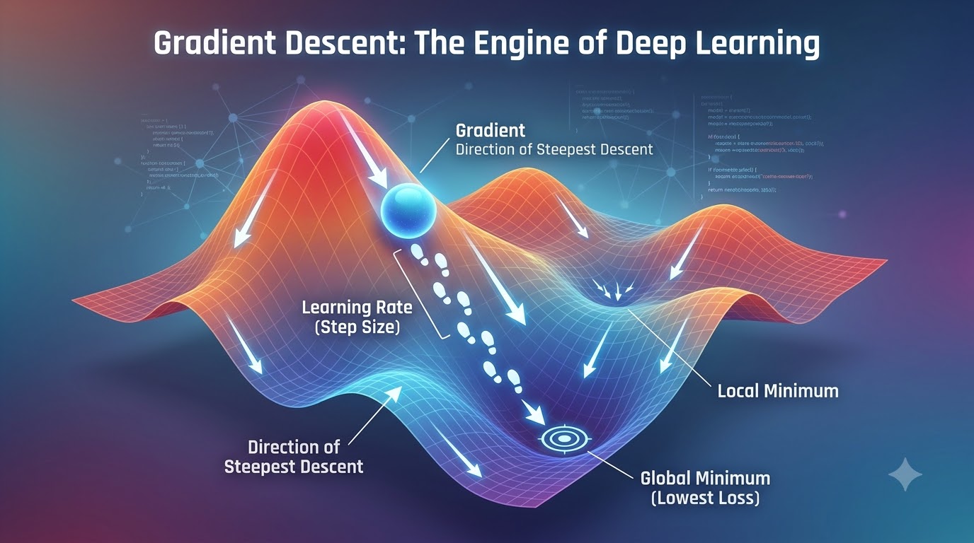
Gradient Descent stands as a cornerstone optimization algorithm in the vast landscape of machine learning and deep learning. It is the fundamental mechanism that allows models to learn from data. This powerful technique iteratively adjusts a model's internal parameters to minimize the difference between its predictions and the actual outcomes.

Think of Gradient Descent as the 'engine' that drives model learning, enabling neural networks to become increasingly accurate over time. Without it, our complex AI systems would struggle to find the optimal configurations needed for tasks like image recognition or natural language processing. Understanding Gradient Descent is crucial for anyone diving into the mechanics of modern AI.

What is Gradient Descent? The Optimization Engine

At its core, Gradient Descent is an optimization algorithm designed to find the minimum of a function. In machine learning, this function is typically the 'loss function' or 'cost function,' which quantifies how well a model performs. A lower loss value indicates a better-performing model.

Imagine you are blindfolded on a foggy mountain and want to reach the lowest point in the valley. You can only feel the slope directly beneath your feet. To descend, you would take a step in the direction of the steepest decline.

This analogy perfectly illustrates Gradient Descent. The 'slope' is the gradient, telling you the direction of the steepest ascent (or descent if you move in the opposite direction). Your 'step size' is controlled by the learning rate, determining how far you move in that direction.

Gradients and Loss Functions: Navigating the Error Landscape

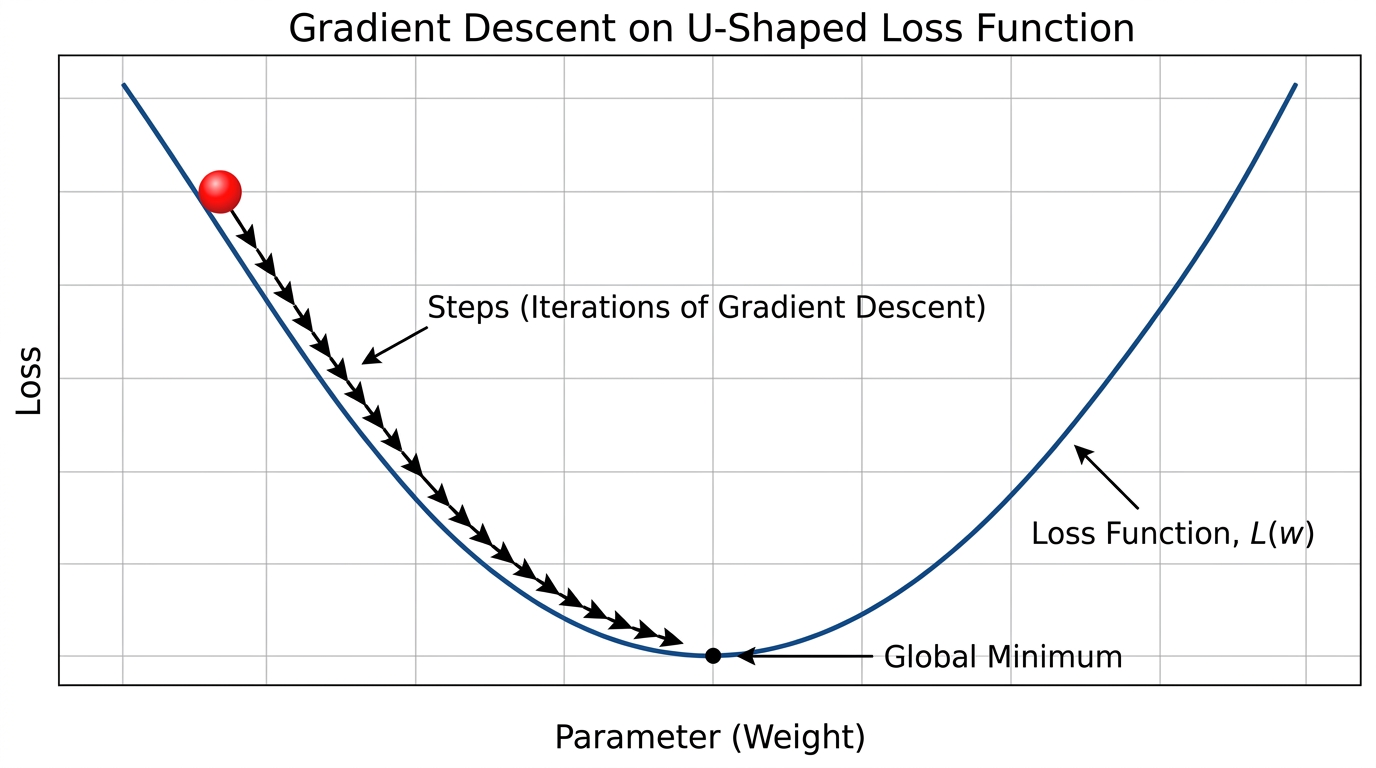
Neural networks, especially deep ones, can have thousands or even millions of adjustable parameters (weights and biases). Optimizing these parameters manually to minimize prediction error is an impossible task. This is precisely why an algorithm like Gradient Descent is indispensable.

The 'loss function' measures the discrepancy between a model's predicted output and the true output. For example, in a regression task, it might be the mean squared error. The goal is always to find the set of parameters that results in the smallest possible loss.

A 'gradient' is a vector that points in the direction of the steepest increase of the loss function. When we apply Gradient Descent, we move in the opposite direction of the gradient. This ensures we are always heading towards a lower loss value, effectively reducing the model's error.

The Core Gradient Descent Formula Explained

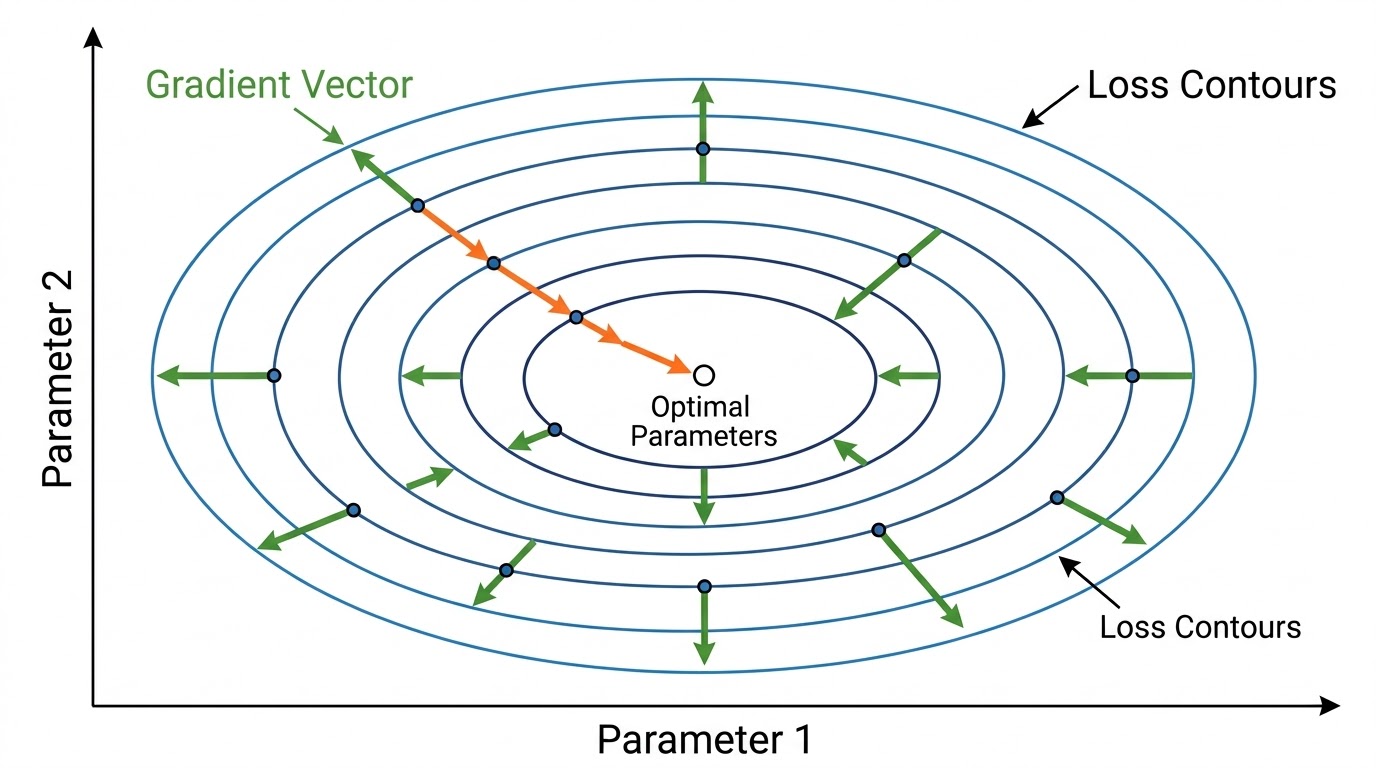
The heart of Gradient Descent lies in its parameter update rule. This simple yet powerful formula dictates how each parameter of the model is adjusted in every iteration. It ensures that the model gradually moves towards a state of lower error.

The core equation for updating a single parameter (theta) is: new_parameter = current_parameter - learning_rate * gradient. Let's break down each component to understand its role in the optimization process.

Here, current_parameter is the current value of the model's weight or bias. The learning_rate is a small positive number that controls the step size. Finally, gradient is the derivative of the loss function with respect to the current parameter, indicating the slope.

# Simple numerical example of a single parameter update

# Assume a simple loss function L(theta) = theta^2
# The derivative (gradient) dL/d(theta) = 2 * theta

current_parameter = 5.0 # Initial parameter value
learning_rate = 0.1     # How big of a step to take

# Calculate the gradient at the current parameter value
gradient = 2 * current_parameter # For L(theta) = theta^2, gradient is 2*theta

# Update the parameter
new_parameter = current_parameter - learning_rate * gradient

print(f"Current Parameter: {current_parameter")
print(f"Calculated Gradient: {gradient")
print(f"Learning Rate: {learning_rate")
print(f"New Parameter: {new_parameter")

# Output:
# Current Parameter: 5.0
# Calculated Gradient: 10.0
# Learning Rate: 0.1
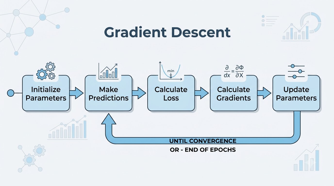
# New Parameter: 4.0

Step-by-Step: How Gradient Descent Works in Practice

Gradient Descent is an iterative process, meaning it repeats a series of steps until a satisfactory solution is found. This cycle allows the model to progressively refine its parameters and improve its performance. Understanding these steps is key to grasping how deep learning models learn.

Here's a breakdown of the complete process:

1. Initialize Parameters: Start by assigning random values to the model's weights and biases. These initial values are typically small and close to zero, providing a starting point for the optimization. This random initialization helps break symmetry and allows different neurons to learn distinct features.
2. Make Predictions: Feed the training data through the model with the current parameters to generate predictions. This is the 'forward pass' of the neural network, where inputs are transformed through layers to produce an output. The initial predictions will likely be far from accurate.
3. Calculate the Loss: Compare the model's predictions with the actual target values using a chosen loss function. This step quantifies the error or discrepancy, giving us a numerical measure of how poorly the model is currently performing. A higher loss means greater error.
4. Calculate Gradients: Compute the gradient of the loss function with respect to each parameter. This step determines the direction and magnitude of change needed for each weight and bias to reduce the loss. For neural networks, this is efficiently done using backpropagation.
5. Update Parameters: Adjust each parameter by subtracting the product of the learning rate and its corresponding gradient. This moves the parameters in the direction that minimizes the loss. The learning rate ensures these adjustments are not too drastic.
6. Repeat Until Convergence: Steps 2-5 are repeated for a fixed number of iterations (epochs) or until the loss function stops decreasing significantly. This iterative refinement allows the model to gradually converge towards an optimal set of parameters, where the loss is minimized.

Exploring Gradient Descent Variants: Batch, SGD, and Mini-Batch

While the core idea of Gradient Descent remains the same, how much data is used to calculate the gradient in each update step leads to different variants. These variants offer trade-offs in terms of computational cost, convergence speed, and stability. Choosing the right variant can significantly impact training efficiency.

The three primary types are Batch Gradient Descent, Stochastic Gradient Descent (SGD), and Mini-Batch Gradient Descent. Each has its own characteristics that make it suitable for different scenarios. Understanding these differences is crucial for practical deep learning applications.

The Learning Rate: Steering Your Model to Success

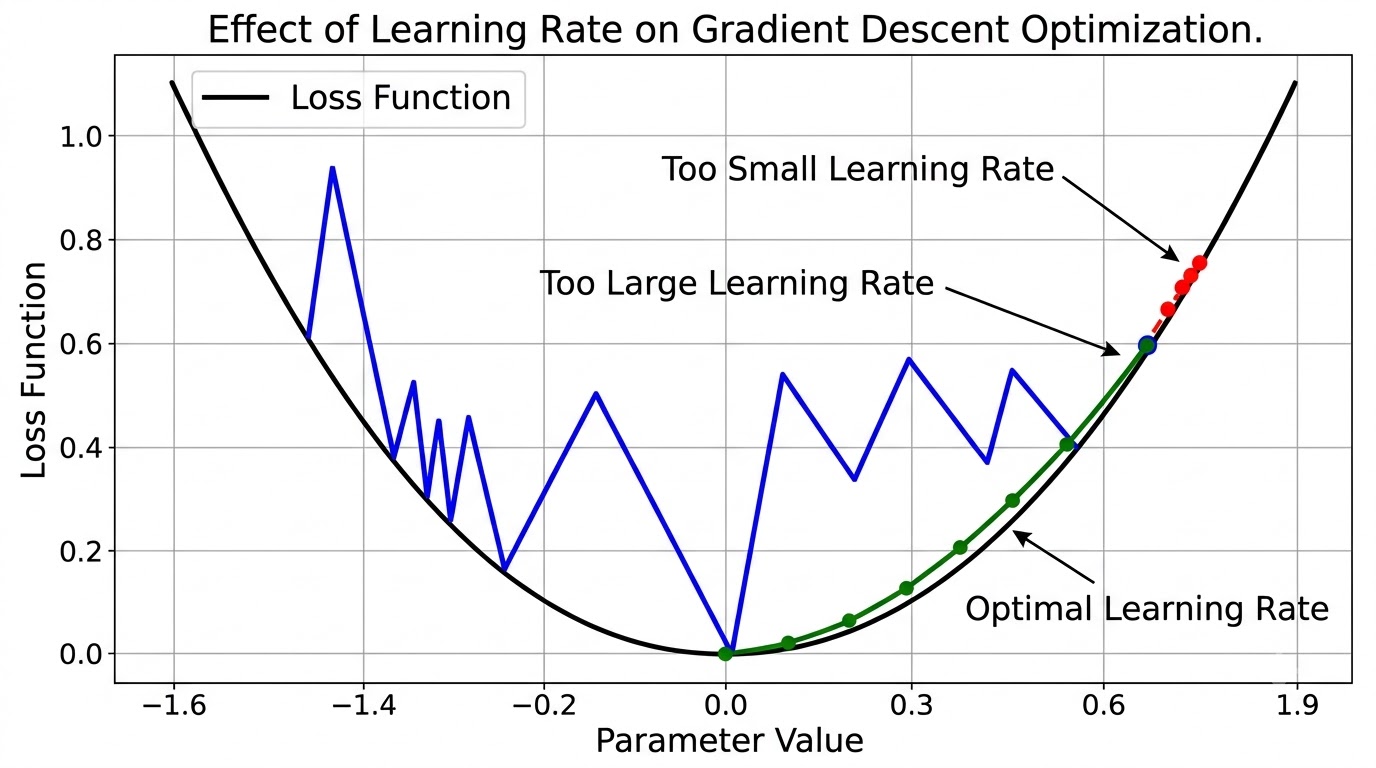
The learning rate is arguably the most critical hyperparameter in Gradient Descent. It controls the step size taken during each parameter update. A carefully chosen learning rate is essential for efficient and effective model training.

An inappropriately chosen learning rate can lead to significant problems. If the learning rate is too small, the model will take tiny steps, resulting in extremely slow convergence. Training might take an unacceptably long time, or it might get stuck before reaching the optimal solution.

Conversely, a learning rate that is too large can cause the optimization process to overshoot the minimum. The model's parameters might oscillate wildly or even diverge, never settling on a stable solution. Finding the 'sweet spot' is often a process of trial and error, or using adaptive learning rate methods.

Gradient Descent and Backpropagation: A Powerful Partnership

While often discussed together, Gradient Descent and Backpropagation play distinct yet complementary roles in training neural networks. Gradient Descent is the overarching optimization algorithm that dictates how parameters are updated. Backpropagation is the specific technique used to calculate the gradients needed for those updates.

Backpropagation efficiently computes the gradient of the loss function with respect to every weight and bias in the network, working backward from the output layer. Once these gradients are calculated, Gradient Descent then takes over, using these values to adjust the parameters. This powerful partnership allows complex neural networks to learn effectively.

Gradient Descent in Action: A Python Tutorial

Let's see Gradient Descent in action by fitting a simple linear regression model to synthetic data. We'll manually calculate gradients and update parameters to illustrate the core mechanics. This example will provide a concrete understanding of the iterative process.

Our goal is to find the best m (slope) and b (intercept) for the equation y = mx + b that minimizes the Mean Squared Error (MSE) loss. We will generate some noisy linear data and then apply Gradient Descent to find the optimal m and b.

import numpy as np
import matplotlib.pyplot as plt

# 1. Generate synthetic data
np.random.seed(42)
X = 2 * np.random.rand(100, 1)
y = 4 + 3 * X + np.random.randn(100, 1) * 1.5 # y = 4 + 3x + noise

# 2. Initialize parameters (m and b)
m = np.random.randn(1, 1) # Slope
b = np.random.randn(1, 1) # Intercept

learning_rate = 0.01
nᵢterations = 1000

# Store loss for plotting
loss_history = []

print(f"Initial m: {m[0][0]:.4f, Initial b: {b[0][0]:.4f")

for iteration in range(nᵢterations):
    # Make predictions
    y_pred = X @ m + b

    # Calculate the loss (Mean Squared Error)
    loss = np.mean((y_pred - y)**2)
    loss_history.append(loss)

    # Calculate gradients
    # Gradient of MSE with respect to m: (2/N) * sum(X * (y_pred - y))
    # Gradient of MSE with respect to b: (2/N) * sum(y_pred - y)
    gradients_m = (2/len(X)) * X.T @ (y_pred - y)
    gradients_b = (2/len(X)) * np.sum(y_pred - y)

    # Update parameters
    m = m - learning_rate * gradients_m
    b = b - learning_rate * gradients_b

print(f"Final m: {m[0][0]:.4f, Final b: {b[0][0]:.4f")

# Plotting the results
plt.figure(figsize=(10, 5))

plt.subplot(1, 2, 1)
plt.scatter(X, y, label='Original Data')
plt.plot(X, X @ m + b, color='red', label='Fitted Line')
plt.title('Linear Regression with Gradient Descent')
plt.xlabel('X')
plt.ylabel('y')
plt.legend()

plt.subplot(1, 2, 2)
plt.plot(loss_history)
plt.title('Loss over Iterations')
plt.xlabel('Iteration')
plt.ylabel('MSE Loss')

plt.tight_layout()
plt.show()

While the manual approach is illustrative, in real-world scenarios, machine learning libraries abstract away these details. Libraries like Scikit-learn, TensorFlow, and PyTorch provide highly optimized implementations of Gradient Descent and its variants. They handle the gradient calculations and parameter updates efficiently.

# Example using Scikit-learn (which uses an optimized solver, often GD-based)
from sklearn.linear_model import LinearRegression

# Continued from previous block - requires X and y setup

model_sklearn = LinearRegression()
model_sklearn.fit(X, y)

print(f"\nScikit-learn m: {model_sklearn.coef_[0][0]:.4f, Scikit-learn b: {model_sklearn.intercept_[0]:.4f")

# Example using TensorFlow/Keras (conceptual, for a simple linear model)
import tensorflow as tf

# Continued from previous block - requires X and y setup

# Define a simple linear model
model_tf = tf.keras.Sequential([
    tf.keras.layers.Dense(units=1, input_shape=[1])
])

# Compile the model with an optimizer (e.g., SGD)
model_tf.compile(optimizer=tf.keras.optimizers.SGD(learning_rate=0.01), loss='mse')

# Train the model
# model_tf.fit(X, y, epochs=1000, verbose=0)

# print(f"TensorFlow m: {model_tf.layers[0].get_weights()[0][0][0]:.4f, TensorFlow b: {model_tf.layers[0].get_weights()[1][0]:.4f")
# Note: To run this, uncomment the fit and print lines. Output will vary slightly due to random initialization and training process.

Common Challenges and Solutions in Gradient Descent

Despite its power, Gradient Descent is not without its challenges. Practitioners often encounter issues that can hinder training efficiency and model performance. Recognizing these problems is the first step toward implementing effective solutions.

Common issues include slow convergence, especially with a poorly chosen learning rate or in flat regions of the loss landscape. Getting stuck in local minima or saddle points can prevent the model from reaching the global optimum. These points can trap the optimization process, leading to suboptimal model performance.

Furthermore, vanishing gradients (where gradients become extremely small) and exploding gradients (where gradients become excessively large) are significant problems in deep neural networks. Vanishing gradients can halt learning in earlier layers, while exploding gradients can lead to unstable training and numerical overflow, making the model unable to learn effectively.

Beyond Basic Gradient Descent: Advanced Optimizers

To address the limitations of basic Gradient Descent, many advanced optimizers have been developed. These optimizers build upon the core algorithm by introducing adaptive learning rates, momentum, or other mechanisms. They aim to achieve faster convergence, greater stability, and better generalization.

Optimizers like Momentum help accelerate Gradient Descent in the relevant direction and dampen oscillations. AdaGrad and RMSProp adapt the learning rate for each parameter individually, scaling it down for parameters with large gradients and up for those with small gradients. This helps navigate complex loss landscapes more effectively.

Adam (Adaptive Moment Estimation) combines the best aspects of Momentum and RMSProp, making it one of the most popular and robust optimizers in deep learning. It computes adaptive learning rates for each parameter and also incorporates a momentum-like term. These advanced optimizers are often the default choice for training state-of-the-art models.

Gradient Descent's Impact on Real-World Deep Learning

The theoretical elegance of Gradient Descent translates directly into its pervasive use across virtually every domain of deep learning. It is the fundamental algorithm that enables neural networks to learn from vast amounts of data. Without it, the breakthroughs we see today would not be possible.

In image classification, Gradient Descent trains models to recognize objects and patterns in images, powering applications from medical diagnostics to autonomous vehicles. For natural language processing, it helps models understand and generate human language, driving advancements in chatbots, translation, and sentiment analysis. Speech recognition systems also rely on Gradient Descent to learn to transcribe spoken words accurately.

Furthermore, recommendation systems use it to learn user preferences, and generative AI models, like those creating realistic images or text, are trained using Gradient Descent to minimize complex objective functions. Its adaptability and efficiency make it the backbone of modern artificial intelligence.

Conclusion: The Enduring Power of Gradient Descent

Gradient Descent is far more than just a mathematical formula; it is the core mechanism that empowers machine learning models to learn and adapt. By iteratively adjusting parameters to minimize prediction error, it enables the complex learning processes that define modern AI. Its foundational role makes it indispensable for anyone working with deep learning.

From its basic principles to its advanced variants, Gradient Descent underpins the success of neural networks across countless applications. Understanding its mechanics, its partnership with Backpropagation, and the role of concepts like loss functions and learning rates, opens the door to deeper insights into the world of artificial intelligence. Continue exploring these interconnected topics to master the art of building intelligent systems.