Artificial Neural Networks (ANN) Explained: Concepts & Code

Introduction to Artificial Neural Networks (ANNs)

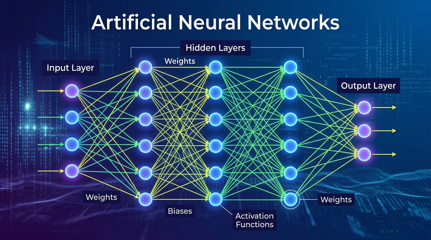
Artificial Neural Networks (ANNs) are computational models inspired by the intricate structure and function of the human brain. They represent a cornerstone of modern Artificial Intelligence, enabling machines to learn, adapt, and make intelligent decisions.

These powerful systems are designed to recognize complex patterns and relationships within vast datasets, often surpassing traditional algorithms in performance. ANNs are fundamental to the advancements seen in machine learning and deep learning today.

Their ability to process information in a way that mimics biological neural networks has led to revolutionary applications across diverse industries, from healthcare to finance and autonomous systems.

What Exactly is an Artificial Neural Network?

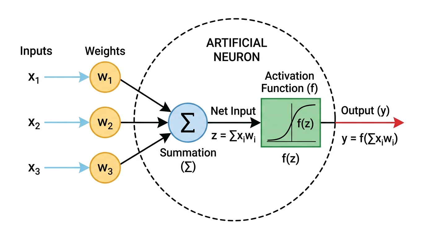
At its core, an Artificial Neural Network is a collection of interconnected processing units called 'neurons' or 'nodes'. Each artificial neuron is a mathematical function that takes one or more inputs, performs a computation, and produces an output.

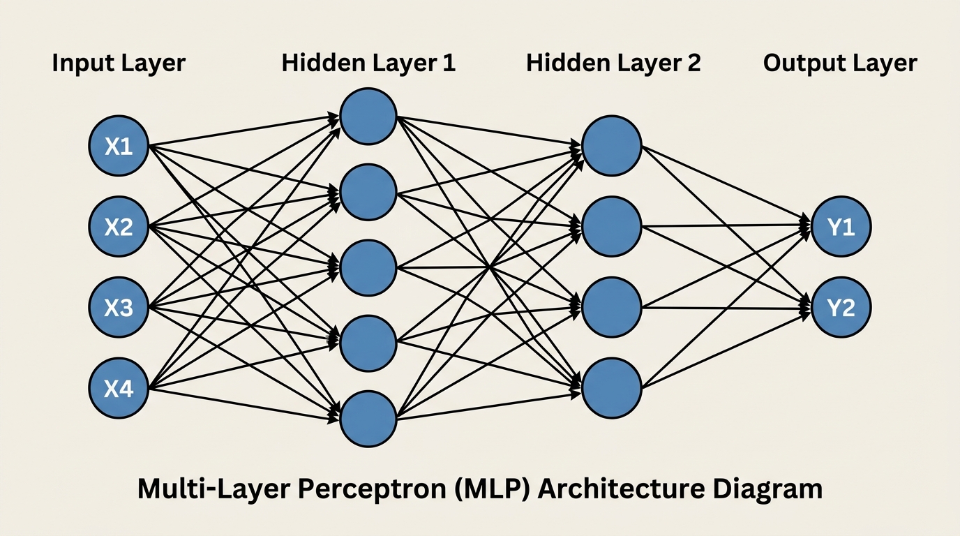
These neurons are organized into layers: an input layer, one or more hidden layers, and an output layer. Information flows from the input layer, through the hidden layers, and finally to the output layer.

Connections between neurons have associated 'weights' and 'biases'. Weights determine the strength of a connection, while biases allow the activation function to be shifted. These parameters are adjusted during the learning process to improve the network's predictions.

A Brief History of Neural Networks: From Perceptrons to Deep Learning

The journey of neural networks began decades ago, evolving from simple models to the complex deep learning architectures we see today. Early pioneers laid the theoretical groundwork, even before computational power could fully realize their potential.

Key breakthroughs in algorithms and hardware have propelled ANNs into the forefront of AI research and application. Understanding this history helps appreciate the iterative nature of scientific progress.

Core Components of an Artificial Neural Network

An ANN is structured into several distinct layers, each serving a specific purpose in processing information. These layers work in concert to transform raw input data into meaningful outputs.

Understanding these components is crucial for designing and interpreting neural network models. Each element plays a vital role in the network's ability to learn and make predictions.

Let's break down the fundamental building blocks:

• Input Layer: This is the entry point for your data. Each neuron in this layer corresponds to a feature in your input dataset. It simply passes the input values to the next layer without performing any complex computations.
• Hidden Layers: These layers are where the magic happens. They perform complex computations and transformations on the input data. A network can have one or many hidden layers, with 'deep' networks having multiple layers.
• Output Layer: This layer produces the final result of the network's computations. The number of neurons here depends on the problem type; for example, one neuron for binary classification or multiple for multi-class classification.
• Neurons (Nodes): Each neuron receives inputs, applies weights, sums them up, adds a bias, and then passes the result through an activation function. This output then becomes an input to neurons in the subsequent layer.
• Weights: These are numerical values assigned to the connections between neurons. They determine the strength or importance of each input connection. Weights are adjusted during the training process to minimize prediction errors.
• Biases: A bias term is added to the weighted sum of inputs before the activation function is applied. It allows the activation function to be shifted, providing more flexibility to the model in fitting the data.
• Activation Functions: These non-linear functions introduce non-linearity into the network, allowing it to learn complex patterns. Without them, an ANN would only be able to learn linear relationships, severely limiting its capabilities.

How Artificial Neural Networks Learn: The Training Process

The true power of an ANN lies in its ability to learn from data, much like a student learns from examples. This learning process involves iteratively adjusting the network's internal parameters to improve its performance on a given task.

It's a cycle of making predictions, evaluating errors, and then making corrections. This iterative refinement allows the network to gradually become more accurate.

The training process can be broken down into several key steps:

Forward Propagation: The Flow of Information

Forward propagation is the initial phase where input data travels through the network from the input layer to the output layer. Each neuron in a layer receives inputs from the previous layer, applies its weights, sums them, adds a bias, and then passes the result through an activation function.

This process generates an output prediction from the network. Think of it like data flowing through a pipeline, being transformed at each stage until a final result emerges.

Calculating Loss and Error: Measuring Performance

Once the network produces an output, we need to compare it to the actual, correct target output. This comparison is done using a 'loss function' (also known as a cost function or error function).

The loss function quantifies the discrepancy between the network's prediction and the true value. Common loss functions include Mean Squared Error (MSE) for regression and Cross-Entropy for classification tasks.

A higher loss value indicates a poorer prediction, while a lower value signifies better accuracy. The goal of training is to minimize this loss.

Backpropagation: Adjusting Weights for Better Predictions

Backpropagation is the core algorithm that enables ANNs to learn efficiently. After calculating the loss, backpropagation works backward from the output layer to the input layer.

It calculates the 'gradient' of the loss function with respect to each weight and bias in the network. The gradient tells us how much each weight and bias contributed to the error and in which direction they should be adjusted to reduce that error.

These calculated gradients are then used by an optimizer (like Gradient Descent) to update the weights and biases. This iterative adjustment process continues over many training examples until the network's predictions are sufficiently accurate.

Key Activation Functions and Their Applications

Activation functions are crucial non-linear components within neurons that determine whether a neuron should be 'activated' or not. They introduce the non-linearity necessary for ANNs to learn complex, non-linear relationships in data.

Without activation functions, even a deep neural network would behave like a simple linear model, severely limiting its expressive power. Different activation functions have distinct properties and are suited for various scenarios.

Diverse Types of Neural Networks and Their Use Cases

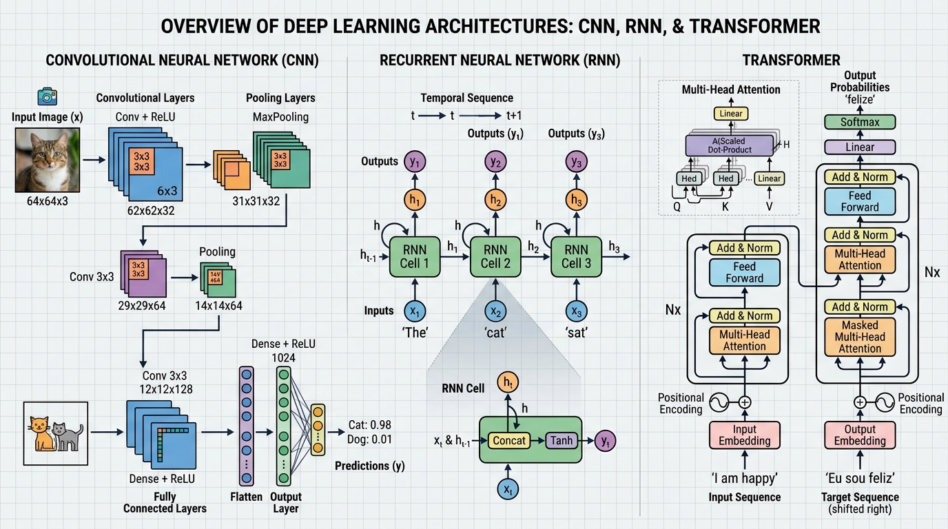
While the basic Feedforward Neural Network (FNN) or Multi-Layer Perceptron (MLP) forms the foundation, many specialized architectures have emerged to tackle specific types of data and problems. These variations are optimized for different tasks.

Each architecture introduces unique mechanisms to process information more effectively for its intended domain. Understanding these distinctions is key to selecting the right tool for your AI project.

Here are some prominent types:

• Feedforward Neural Networks (FNNs) / Multi-Layer Perceptrons (MLPs): The simplest form, where information flows in one direction from input to output. Used for classification, regression, and pattern recognition on tabular data.
• Convolutional Neural Networks (CNNs): Designed specifically for processing grid-like data, such as images. They use convolutional layers to automatically learn spatial hierarchies of features, making them highly effective for computer vision tasks.
• Recurrent Neural Networks (RNNs): Built to handle sequential data, where the order of information matters. RNNs have internal memory, allowing them to process sequences like text, speech, and time series data. However, they struggle with long-term dependencies.
• Long Short-Term Memory (LSTMs): A special type of RNN designed to overcome the vanishing gradient problem and better capture long-term dependencies in sequential data. Widely used in natural language processing and speech recognition.
• Transformers: A revolutionary architecture that relies on self-attention mechanisms to weigh the importance of different parts of the input sequence. They have become the state-of-the-art for many NLP tasks, including machine translation and text generation.

Training an ANN: Datasets, Epochs, and Optimizers

Training an ANN involves more than just forward and backpropagation; it requires careful consideration of data, training parameters, and optimization strategies. These practical aspects significantly influence the model's performance and generalization ability.

Proper data preparation and hyperparameter tuning are critical steps in developing robust neural network models. Let's explore the key elements involved in the training process.

• Datasets: Data is typically split into three sets: a training set (used to train the model), a validation set (used to tune hyperparameters and prevent overfitting during training), and a test set (used for final, unbiased evaluation of the model's performance).
• Epochs: An epoch represents one complete pass through the entire training dataset. During each epoch, the network processes all training examples, performs forward propagation, calculates loss, and updates weights via backpropagation.
• Batch Size: Instead of updating weights after every single training example, data is often processed in 'batches'. Batch size refers to the number of training examples processed before the network's weights are updated. Smaller batches introduce more noise but can help escape local minima, while larger batches provide a more stable gradient estimate.
• Learning Rate: This hyperparameter controls how much the weights are adjusted with respect to the loss gradient during backpropagation. A high learning rate can cause the model to overshoot the optimal weights, while a low learning rate can make training very slow.
• Optimizers: Optimizers are algorithms that adjust the learning rate and update the network's weights and biases more effectively. Popular optimizers include Stochastic Gradient Descent (SGD), Adam, RMSprop, and Adagrad. They help navigate the complex loss landscape to find optimal parameters.
• Loss Functions: As discussed, loss functions quantify the error between predicted and actual values. The choice of loss function is critical and depends on the specific task (e.g., binary cross-entropy for binary classification, categorical cross-entropy for multi-class classification, mean squared error for regression).

Advantages and Limitations of Artificial Neural Networks

Artificial Neural Networks have revolutionized many fields, offering unparalleled capabilities in pattern recognition and complex data analysis. However, like any powerful technology, they come with their own set of challenges and limitations.

A balanced understanding of both their strengths and weaknesses is essential for effective and responsible deployment. Let's explore the key advantages and limitations.

Advantages:

• Pattern Recognition: ANNs excel at identifying intricate, non-linear patterns in data that are often imperceptible to humans or traditional algorithms. This makes them ideal for tasks like image and speech recognition.
• Adaptability and Learning: They can learn from examples and adapt their internal structure (weights and biases) to new data without being explicitly reprogrammed. This makes them highly flexible and robust.
• Handling Complex Relationships: ANNs can model highly complex, non-linear relationships between inputs and outputs, which is crucial for real-world problems where data is rarely linearly separable.
• Fault Tolerance: Due to their distributed nature, ANNs can exhibit a degree of fault tolerance. If a few neurons or connections fail, the network can often still function reasonably well.
• Generalization: A well-trained ANN can generalize well to unseen data, making accurate predictions on new examples it has not encountered during training.

Limitations:

• Computational Requirements: Training deep ANNs, especially with large datasets, requires significant computational power (GPUs, TPUs) and time. Inference can also be resource-intensive for complex models.
• Data Dependency: ANNs are highly data-hungry. They require vast amounts of high-quality, labeled training data to learn effectively. Insufficient or biased data can lead to poor performance.
• 'Black Box' Interpretability: Complex ANNs are often considered 'black boxes' because it's difficult to understand exactly how they arrive at a particular decision. This lack of transparency can be a major concern in critical applications like healthcare or finance.
• Hyperparameter Tuning: Designing an ANN involves choosing many hyperparameters (e.g., number of layers, neurons per layer, learning rate, activation functions). Optimal tuning is often a trial-and-error process and can be very time-consuming.
• Overfitting: ANNs can easily overfit the training data, meaning they learn the training examples too well, including their noise, and fail to generalize to new, unseen data. Regularization techniques are needed to mitigate this.

Real-World Applications Powered by ANNs

Artificial Neural Networks are no longer just a theoretical concept; they are deeply embedded in the technologies we use every day. Their ability to process complex data has led to transformative applications across nearly every sector.

From enhancing user experiences to solving critical scientific challenges, ANNs are driving innovation. Here are some compelling examples of their widespread impact.

• Image Recognition: Powering facial recognition in smartphones, object detection in autonomous vehicles, and medical image analysis for disease diagnosis. CNNs are particularly effective here.
• Speech Recognition: Enabling voice assistants like Siri, Alexa, and Google Assistant, as well as transcription services. RNNs and Transformers play a crucial role in understanding spoken language.
• Recommendation Systems: Driving personalized recommendations on platforms like Netflix (movies), Amazon (products), and Spotify (music), by predicting user preferences based on past behavior.
• Fraud Detection: Identifying anomalous transactions in banking and credit card systems, flagging potential fraudulent activities in real-time. ANNs can detect subtle patterns indicative of fraud.
• Healthcare: Assisting in disease diagnosis (e.g., detecting tumors in X-rays), drug discovery, and personalized treatment plans by analyzing patient data.
• Autonomous Vehicles: Processing sensor data from cameras, lidar, and radar to perceive the environment, navigate, and make driving decisions. This involves complex object detection and prediction tasks.
• Natural Language Processing (NLP): Powering machine translation, sentiment analysis, chatbots, and text summarization. Transformers have significantly advanced the capabilities in this domain.

Building Your First ANN with Python (TensorFlow/Keras)

Now that we've covered the theoretical foundations, let's get hands-on and build a simple Artificial Neural Network using Python. We'll leverage TensorFlow and its high-level Keras API, which makes building neural networks straightforward.

We'll tackle a classic classification problem, such as classifying different species of Iris flowers based on their measurements. This example will walk you through the entire process, from data preparation to model evaluation.

Setting Up Your Python Environment

First, ensure you have Python installed (version 3.9+ is recommended). It's good practice to use a virtual environment to manage your project dependencies.

Open your terminal or command prompt and follow these steps to create a virtual environment and install the necessary libraries.

python -m venv ann_env
source ann_env/bin/activate  # On Windows, use `ann_env\Scripts\activate`
pip install tensorflow scikit-learn numpy pandas matplotlib

Data Preprocessing for Classification

We'll use the famous Iris dataset, which is readily available in Scikit-learn. This dataset contains measurements of three different species of Iris flowers.

Preprocessing involves loading the data, splitting it into training and testing sets, and then scaling the features. For the target labels, we'll use one-hot encoding, which converts categorical labels into a binary vector format suitable for neural networks.

import numpy as np
import pandas as pd
from sklearn.datasets import loadᵢris
from sklearn.model_selection import train_test_split
from sklearn.preprocessing import StandardScaler, OneHotEncoder
from tensorflow.keras.utils import to_categorical

# Load the Iris dataset
iris = loadᵢris()
X = iris.data
y = iris.target

# Split data into training and testing sets
X_train, X_test, y_train, y_test = train_test_split(X, y, test_size=0.2, random_state=42)

# Feature Scaling
# Standardize features by removing the mean and scaling to unit variance
scaler = StandardScaler()
X_train_scaled = scaler.fit_transform(X_train)
X_test_scaled = scaler.transform(X_test)

# One-hot encode target labels
# Converts integer labels (0, 1, 2) into binary vectors (e.g., [1,0,0], [0,1,0])
encoder = OneHotEncoder(sparse_output=False)
y_train_encoded = encoder.fit_transform(y_train.reshape(-1, 1))
y_test_encoded = encoder.transform(y_test.reshape(-1, 1))

print(f"X_train_scaled shape: {X_train_scaled.shape")
print(f"y_train_encoded shape: {y_train_encoded.shape")
print(f"Number of features: {X_train_scaled.shape[1]")
print(f"Number of classes: {y_train_encoded.shape[1]")

Designing and Compiling the ANN Model

Now, we'll define our Artificial Neural Network using Keras's Sequential API. This allows us to build a model layer by layer. We'll create a simple feedforward network with one input layer, two hidden layers, and an output layer.

We'll specify the number of neurons, activation functions for each layer, and then compile the model with an optimizer and a loss function suitable for multi-class classification. The model.summary() command provides a useful overview of the network architecture.

import tensorflow as tf
from tensorflow.keras.models import Sequential
from tensorflow.keras.layers import Dense

# Define the ANN model
model = Sequential([
    # Input layer and first hidden layer
    # input_shape specifies the number of features in the input data
    Dense(units=10, activation='relu', input_shape=(X_train_scaled.shape[1],)),
    # Second hidden layer
    Dense(units=8, activation='relu'),
    # Output layer
    # units is the number of classes, activation='softmax' for multi-class classification
    Dense(units=y_train_encoded.shape[1], activation='softmax')
])

# Compile the model
# optimizer: Adam is a popular choice for its efficiency
# loss: categorical_crossentropy for multi-class classification with one-hot encoded labels
# metrics: accuracy to monitor performance during training
model.compile(optimizer='adam', loss='categorical_crossentropy', metrics=['accuracy'])

# Print model summary to see the architecture and number of parameters
model.summary()

Training and Evaluating the ANN

With the model defined and compiled, the next step is to train it using our preprocessed training data. We'll use the model.fit() method, specifying the training data, number of epochs, and batch size.

After training, we evaluate the model's performance on the unseen test set using model.evaluate(). This gives us an unbiased measure of how well our ANN generalizes to new data. We'll print the final test loss and accuracy.

# Continued from previous block - requires the setup and model definition above

# Train the model
# epochs: number of times the model will iterate over the entire training dataset
# batch_size: number of samples per gradient update
print("\nTraining the model...")
history = model.fit(
    X_train_scaled, y_train_encoded,
    epochs=100,
    batch_size=16,
    verbose=0 # Set to 1 or 2 for more detailed output during training
)

# Evaluate the model on the test set
print("\nEvaluating the model...")
loss, accuracy = model.evaluate(X_test_scaled, y_test_encoded, verbose=0)

print(f"Test Loss: {loss:.4f")
print(f"Test Accuracy: {accuracy:.4f")

# You can also plot the training history to visualize loss and accuracy over epochs
import matplotlib.pyplot as plt

plt.figure(figsize=(12, 5))

plt.subplot(1, 2, 1)
plt.plot(history.history['loss'], label='Training Loss')
plt.title('Loss over Epochs')
plt.xlabel('Epoch')
plt.ylabel('Loss')
plt.legend()

plt.subplot(1, 2, 2)
plt.plot(history.history['accuracy'], label='Training Accuracy')
plt.title('Accuracy over Epochs')
plt.xlabel('Epoch')
plt.ylabel('Accuracy')
plt.legend()

plt.tight_layout()
plt.show()

# Example prediction
print("\nMaking a prediction on a sample from the test set:")
sampleᵢndex = 0
sampleᵢnput = X_test_scaled[sampleᵢndex:sampleᵢndex+1]
predicted_probabilities = model.predict(sampleᵢnput)
predicted_class = np.argmax(predicted_probabilities)
true_class = np.argmax(y_test_encoded[sampleᵢndex])

print(f"Sample Input: {iris.featureₙames = {scaler.inverse_transform(sampleᵢnput)[0]")
print(f"Predicted Probabilities: {predicted_probabilities[0]")
print(f"Predicted Class (index): {predicted_class ({iris.targetₙames[predicted_class])")
print(f"True Class (index): {true_class ({iris.targetₙames[true_class])")

Common Mistakes and Pitfalls in ANN Development

Developing Artificial Neural Networks can be challenging, and it's easy to fall into common traps that hinder performance. Recognizing these pitfalls early can save significant time and effort during model development.

Understanding these issues helps in debugging and improving your ANN models. Here are some of the most frequent mistakes and how to identify them.

• Overfitting: Occurs when the model learns the training data too well, including noise and specific details, leading to poor performance on unseen data. The model essentially memorizes the training set rather than learning general patterns.
• Underfitting: Happens when the model is too simple to capture the underlying patterns in the data. It performs poorly on both training and test sets, indicating it hasn't learned enough from the data.
• Vanishing/Exploding Gradients: During backpropagation, gradients can become extremely small (vanishing) or extremely large (exploding). Vanishing gradients prevent deep layers from learning, while exploding gradients lead to unstable training and large weight updates.
• Poor Feature Scaling: If input features have vastly different scales, the optimization algorithm might struggle to converge efficiently. Features with larger values can dominate the learning process, leading to suboptimal weight updates.
• Incorrect Learning Rate: A learning rate that is too high can cause the model to diverge or oscillate around the minimum loss. A learning rate that is too low can make training excessively slow, potentially getting stuck in a local minimum.
• Insufficient Training Data: ANNs are data-hungry. Training a complex model on too little data can lead to overfitting and poor generalization. The model simply doesn't have enough examples to learn robust patterns.

Best Practices for Effective ANN Development

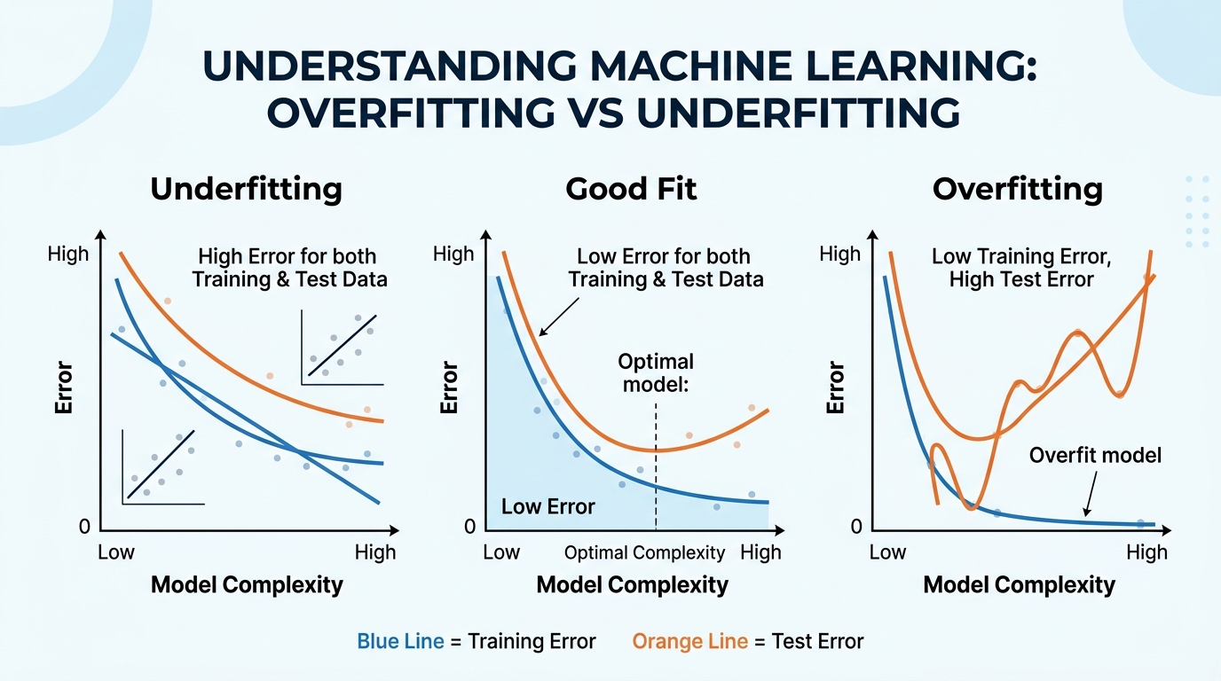
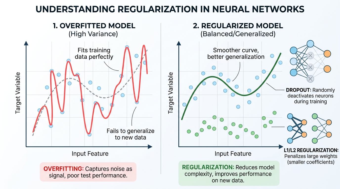
Building high-performing and reliable Artificial Neural Networks requires more than just knowing the components; it demands adherence to best practices throughout the development lifecycle. These practices help ensure your models are robust, efficient, and generalize well.

Adopting these strategies can significantly improve the quality and stability of your ANN projects. Let's explore key recommendations for effective ANN development.

• Thorough Data Preprocessing and Augmentation: Always clean, normalize, and scale your data. For image data, consider augmentation techniques (e.g., rotation, flipping, cropping) to increase the effective size and diversity of your training set, reducing overfitting.
• Appropriate Architecture Selection: Choose an ANN architecture that aligns with your data type and problem. For images, CNNs are typically superior; for sequences, RNNs or Transformers are better. Start with simpler models and gradually increase complexity.
• Regularization Techniques: Combat overfitting using methods like L1/L2 regularization (penalizing large weights) and Dropout (randomly deactivating neurons during training). These force the network to learn more robust features.
• Hyperparameter Tuning: Don't guess hyperparameters. Use systematic approaches like Grid Search, Random Search, or more advanced methods like Bayesian Optimization to find the optimal combination of learning rate, batch size, number of layers, and neurons.
• Early Stopping: Monitor the model's performance on a validation set during training. Stop training when the validation loss starts to increase, even if the training loss is still decreasing. This prevents overfitting.
• Careful Model Evaluation: Beyond accuracy, use appropriate metrics for your problem (e.g., precision, recall, F1-score for imbalanced classification; R-squared for regression). Analyze confusion matrices and learning curves to gain deeper insights into model behavior.
• Initialize Weights Properly: Using appropriate weight initialization techniques (e.g., He initialization for ReLU, Xavier initialization for Tanh/Sigmoid) can significantly speed up training and prevent vanishing/exploding gradients.

Conclusion: The Future of Neural Networks

We've journeyed through the fascinating world of Artificial Neural Networks, from their brain-inspired origins and core components to their learning mechanisms and diverse applications. ANNs are undeniably a cornerstone of modern AI, driving innovation across countless domains.

Their ability to learn complex patterns from data has unlocked capabilities once thought to be science fiction. As computational power grows and new architectures emerge, the potential of neural networks continues to expand at an astonishing pace.

For those eager to explore further, consider diving into specialized architectures like Convolutional Neural Networks for advanced computer vision, Recurrent Neural Networks and Transformers for cutting-edge natural language processing, or delving into ethical AI considerations. The journey into neural networks is an exciting and ever-evolving one.

Dive Deeper with the Code

Ready to roll up your sleeves? Clone the companion repository, explore the full ANN implementation, and tweak the examples to see the concepts in action.

GitHub Repository: Artificial Neural Networks (ANN) Explained: Concepts & Code