>_Programming Partner
Loading technical insights...
Loading technical insights...
Software Developer
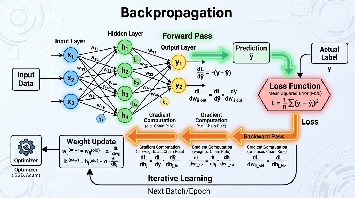
Backpropagation stands as one of the most pivotal algorithms in the realm of deep learning. It is the fundamental mechanism responsible for teaching neural networks how to refine their predictions and improve their performance over time. Without backpropagation, the sophisticated AI models we use today would not be able to learn from data.
This powerful algorithm allows neural networks to adjust their internal parameters based on the errors they make during training. Essentially, it's how a neural network learns from its mistakes, becoming smarter with each iteration. Its efficiency and effectiveness have made it indispensable.
Nearly every modern AI model, from image recognition systems to natural language processors, relies on backpropagation during its training phase. Understanding backpropagation is crucial for anyone looking to grasp the inner workings of deep learning and build intelligent systems.
At its heart, backpropagation is an algorithm that calculates how much each individual neuron in a neural network contributes to the overall prediction error. This calculation is vital because it tells the network which parts need adjustment. It's like a diagnostic tool for the network's learning process.
Once these contributions are quantified, backpropagation systematically adjusts the network's internal weights and biases. These adjustments are made in a way that minimizes the overall loss function, which is a measure of how far off the network's predictions are from the actual values. The goal is to reduce this error as much as possible.
By iteratively minimizing this loss, backpropagation enables neural networks to learn from their mistakes. Over many training cycles, the network becomes increasingly accurate and capable of making reliable predictions on new, unseen data. This continuous refinement is what makes deep learning so powerful.
When a neural network is first created, its internal parameters, known as weights and biases, are typically initialized with random values. This means that the network's initial predictions are essentially guesswork and highly inaccurate. It's like a newborn brain with no prior experience.
Backpropagation provides the systematic method for updating these random weights and biases. It uses the calculated error from the network's predictions to determine how each parameter should be tweaked. This process ensures that the network doesn't just guess, but actively learns from its performance.
Through this iterative adjustment, the model gradually becomes more accurate and gains the ability to generalize well to new data. Each pass through the training data, guided by backpropagation, refines the network's understanding of the underlying patterns. This continuous learning is fundamental to achieving high-performing AI models.
Understanding backpropagation requires familiarity with the core components that make up a neural network. Each element plays a distinct and crucial role in how the network processes information and learns from data. These components work in harmony to facilitate the learning process.
From the basic computational units to the functions that guide learning, each part is essential. Let's explore these fundamental building blocks and their contributions to the overall learning mechanism. This foundational knowledge is key to grasping backpropagation's mechanics.
| Component | Description | Role in Backpropagation |
|---|---|---|
| Neurons | Basic computational units that receive inputs, process them, and produce an output. | Perform weighted sums and apply activation functions; their outputs are used in forward pass, and their internal states are adjusted. |
| Weights | Parameters that determine the strength of the connection between neurons. | Adjusted during backpropagation to minimize error; represent the learned knowledge of the network. |
| Biases | Additional parameters added to the weighted sum, shifting the activation function's output. | Adjusted alongside weights to fine-tune the neuron's activation threshold and improve model fit. |
| Activation Functions | Non-linear functions applied to the weighted sum of inputs, introducing complexity. | Introduce non-linearity, allowing networks to learn complex patterns; their derivatives are crucial for gradient calculation. |
| Loss Function | Measures the discrepancy between the network's predictions and the actual target values. | Quantifies the error that backpropagation aims to minimize; gradients are calculated with respect to this function. |
| Gradients | Vectors of partial derivatives indicating the direction and magnitude of the steepest ascent of the loss function. | Calculated for each weight and bias during the backward pass, guiding the parameter updates. |
| Learning Rate | A hyperparameter that controls the step size during weight updates. | Determines how aggressively weights are adjusted based on gradients; a critical factor for convergence and stability. |
Backpropagation isn't a single step but a carefully orchestrated sequence of operations. It involves both a forward pass, where predictions are made, and a backward pass, where errors are analyzed and parameters are adjusted. This cyclical process is repeated many times.
The entire workflow is designed to systematically reduce the network's prediction error over multiple training iterations, known as epochs. Each epoch refines the network's understanding, making it more accurate. Let's break down this iterative learning cycle.
Understanding this step-by-step process is key to appreciating how neural networks achieve their impressive learning capabilities. It highlights the continuous feedback loop that drives improvement. The diagram below illustrates this flow.
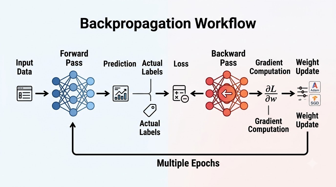
The first stage of the backpropagation workflow is called forward propagation. During this phase, input data is fed into the neural network and travels through its various layers, from the input layer, through hidden layers, and finally to the output layer. This is where the network makes its initial prediction.
Within each neuron, the inputs are multiplied by their respective weights and summed up, along with a bias term. This weighted sum then passes through an activation function, which introduces non-linearity into the network. This non-linearity is crucial for learning complex patterns.
The outputs of one layer become the inputs for the next, until a final prediction is generated at the output layer. At this point, the network has made a guess based on its current weights and biases, but no learning adjustments have occurred yet. This prediction is then ready for evaluation.
After the forward pass generates a prediction, the next critical step is to quantify how accurate that prediction is. This is achieved by comparing the network's output with the actual, correct target values, also known as ground truth. The difference between these two is the error or loss.
A loss function is a mathematical formula that calculates this discrepancy. The primary objective of training a neural network is to minimize this loss function. A smaller loss indicates that the network's predictions are closer to the true values, signifying better performance.
Different types of tasks require different loss functions. For instance, regression problems, where the goal is to predict a continuous value, often use Mean Squared Error. Classification problems, aiming to categorize inputs, commonly employ Cross-Entropy Loss. Understanding the appropriate loss function is vital for effective training.
| Loss Function | Formula | Typical Use Case | Explanation |
|---|---|---|---|
| Mean Squared Error (MSE) | MSE = (1/N) * ∑_i=1^{N (yᵢ - \hat{yᵢ)^2 | Regression | Calculates the average of the squared differences between predicted and actual values. Penalizes larger errors more heavily. |
| Cross-Entropy Loss | CE = -∑_i=1^{C yᵢ \log(\hat{yᵢ) | Classification | Measures the performance of a classification model whose output is a probability value between 0 and 1. Increases as the predicted probability diverges from the actual label. |
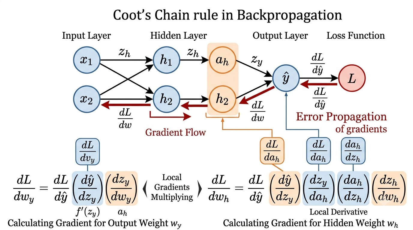
Once the loss is calculated, the network needs to understand how to adjust its weights and biases to reduce this error. This is where gradients come into play. Gradients are essentially measurements of how much each weight and bias in the network affects the overall prediction error.
To compute these gradients efficiently across multiple layers of a neural network, backpropagation leverages a fundamental concept from calculus: the chain rule. The chain rule allows us to calculate the derivative of a composite function by multiplying the derivatives of its individual components. This is crucial for propagating error backward.
Starting from the output layer, the error is propagated backward through the network, layer by layer. At each layer, the chain rule is applied to determine the gradient of the loss with respect to the weights and biases of that specific layer. This systematic approach ensures that every parameter's contribution to the error is precisely quantified.
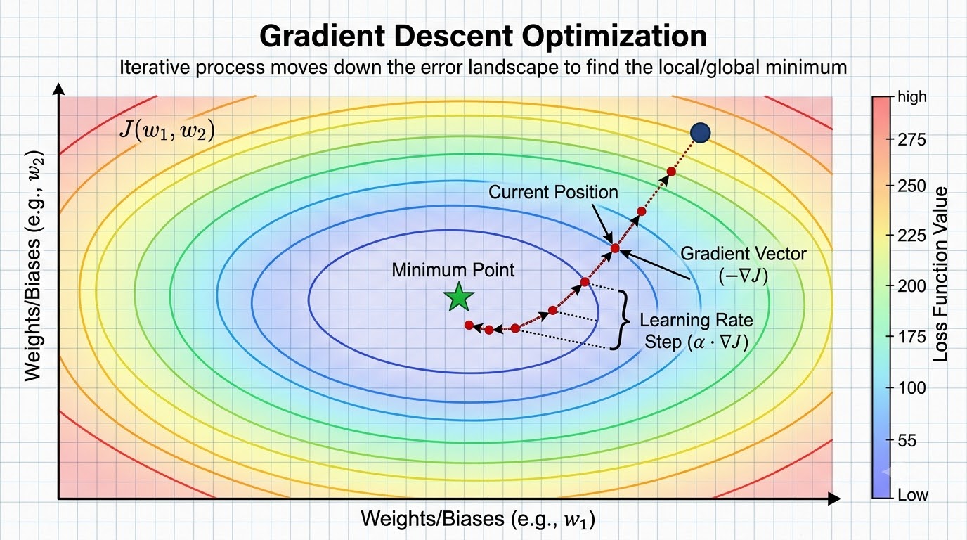
With the gradients calculated for each weight and bias, the network now has the information needed to adjust its parameters. This adjustment is performed by optimization algorithms, with Gradient Descent being the most common. Gradient Descent aims to find the minimum of the loss function.
The algorithm updates the weights and biases by moving them in the opposite direction of their respective gradients. Since gradients point towards the steepest ascent of the loss function, moving in the opposite direction ensures that the loss decreases. This iterative process gradually steers the network towards better performance.
A crucial hyperparameter in this step is the learning rate. The learning rate determines the size of each update step. A small learning rate leads to slow convergence but can be more stable, while a large learning rate can cause the model to overshoot the minimum or even diverge. Choosing an appropriate learning rate is vital for successful training.
Activation functions are non-linear transformations applied to the weighted sum of inputs in a neuron. Without them, a neural network would simply be a series of linear operations, regardless of how many layers it has. This would severely limit its ability to learn complex, non-linear patterns in data.
By introducing non-linearity, activation functions enable the network to model intricate relationships between inputs and outputs. This capacity to learn complex features is what gives deep neural networks their power. They are essential for solving real-world problems that are inherently non-linear.
The choice of activation function also significantly impacts the gradient flow during backpropagation. Some functions can lead to issues like vanishing or exploding gradients, while others are designed to mitigate these problems. Let's compare some commonly used activation functions.
| Activation Function | Mathematical Form | Effect on Gradient Flow | Typical Use Cases |
|---|---|---|---|
| ReLU (Rectified Linear Unit) | f(x) = max(0, x) | For x > 0, gradient is 1; for x <= 0, gradient is 0. Helps mitigate vanishing gradients but can suffer from 'dying ReLU' problem. | Hidden layers in deep neural networks, especially for image processing. |
| Sigmoid | f(x) = 1 / (1 + e^(-x)) | Outputs values between 0 and 1. Gradients are very small for large positive or negative inputs, leading to vanishing gradients. | Output layer for binary classification problems (e.g., predicting probabilities). |
| Tanh (Hyperbolic Tangent) | f(x) = (e^x - e^(-x)) / (e^x + e^(-x)) | Outputs values between -1 and 1. Stronger gradients than Sigmoid but still prone to vanishing gradients for extreme inputs. | Hidden layers, often preferred over Sigmoid due to zero-centered output. |
To solidify our understanding, let's walk through a simplified numerical example of backpropagation. We'll use a very small neural network with one input, one hidden layer with two neurons, and one output neuron. This will demonstrate the forward pass, error calculation, and weight updates.
Imagine our network is trying to learn a simple mapping. We'll use a sigmoid activation function for the hidden layer and the output layer, and Mean Squared Error for the loss. This example will illustrate the core mechanics without excessive complexity.
This step-by-step calculation will show how the error signal is propagated backward to adjust weights. While real-world networks are much larger, the underlying principles remain the same. We'll see how a single training iteration updates the network's parameters.
import numpy as np

def sigmoid(x):
    return 1 / (1 + np.exp(-x))

def sigmoid_derivative(x):
    return x * (1 - x)

# Input data
X = np.array([[0.5]])
# Actual target output
y = np.array([[0.8]])

# Initial weights and biases (randomly initialized)
# Hidden layer weights
W1 = np.array([[0.1, 0.2]])
# Hidden layer biases
b1 = np.array([[0.3, 0.4]])
# Output layer weights
W2 = np.array([[0.5], [0.6]])
# Output layer bias
b2 = np.array([[0.7]])

# Learning rate
learning_rate = 0.1

print("--- Initial State ---")
print(f"Input X: {X")
print(f"Target y: {y")
print(f"W1: {W1, b1: {b1")
print(f"W2: {W2, b2: {b2")

# --- Forward Pass ---
# Hidden layer calculation
# Z1 = X * W1 + b1
Z1 = np.dot(X, W1) + b1
# A1 = sigmoid(Z1)
A1 = sigmoid(Z1)

# Output layer calculation
# Z2 = A1 * W2 + b2
Z2 = np.dot(A1, W2) + b2
# A2 = sigmoid(Z2) (predicted output)
A2 = sigmoid(Z2)

print("\n--- Forward Pass Results ---")
print(f"Hidden layer output (A1): {A1")
print(f"Predicted output (A2): {A2")

# --- Calculate Loss (Mean Squared Error) ---
# Loss = 0.5 * (y - A2)^2
loss = 0.5 * np.sum(np.square(y - A2))
print(f"Loss: {loss")

# --- Backward Pass ---
# Step 1: Calculate gradient of loss with respect to output (A2)
# dLoss/dA2 = -(y - A2)
dLoss_dA2 = -(y - A2)

# Step 2: Calculate gradient of A2 with respect to Z2 (sigmoid derivative)
# dA2/dZ2 = A2 * (1 - A2)
dA2_dZ2 = sigmoid_derivative(A2)

# Step 3: Calculate gradient of loss with respect to Z2
# dLoss/dZ2 = dLoss/dA2 * dA2/dZ2
dLoss_dZ2 = dLoss_dA2 * dA2_dZ2

# Step 4: Calculate gradient of loss with respect to W2
# dLoss/dW2 = A1.T * dLoss/dZ2
dLoss_dW2 = np.dot(A1.T, dLoss_dZ2)

# Step 5: Calculate gradient of loss with respect to b2
# dLoss/db2 = dLoss/dZ2 (summed over batch, if batch > 1)
dLoss_db2 = dLoss_dZ2

# Step 6: Calculate gradient of loss with respect to A1
# dLoss/dA1 = dLoss/dZ2 * W2.T
dLoss_dA1 = np.dot(dLoss_dZ2, W2.T)

# Step 7: Calculate gradient of A1 with respect to Z1 (sigmoid derivative)
# dA1/dZ1 = A1 * (1 - A1)
dA1_dZ1 = sigmoid_derivative(A1)

# Step 8: Calculate gradient of loss with respect to Z1
# dLoss/dZ1 = dLoss/dA1 * dA1/dZ1
dLoss_dZ1 = dLoss_dA1 * dA1_dZ1

# Step 9: Calculate gradient of loss with respect to W1
# dLoss/dW1 = X.T * dLoss/dZ1
dLoss_dW1 = np.dot(X.T, dLoss_dZ1)

# Step 10: Calculate gradient of loss with respect to b1
# dLoss/db1 = dLoss/dZ1 (summed over batch, if batch > 1)
dLoss_db1 = dLoss_dZ1

print("\n--- Gradients ---")
print(f"dLoss_dW1: {dLoss_dW1")
print(f"dLoss_db1: {dLoss_db1")
print(f"dLoss_dW2: {dLoss_dW2")
print(f"dLoss_db2: {dLoss_db2")

# --- Update Weights and Biases (Gradient Descent) ---
W1ₙew = W1 - learning_rate * dLoss_dW1
b1ₙew = b1 - learning_rate * dLoss_db1
W2ₙew = W2 - learning_rate * dLoss_dW2
b2ₙew = b2 - learning_rate * dLoss_db2

print("\n--- Updated Parameters ---")
print(f"Updated W1: {W1ₙew")
print(f"Updated b1: {b1ₙew")
print(f"Updated W2: {W2ₙew")
print(f"Updated b2: {b2ₙew")

# Verify with another forward pass (optional)
# Z1ₙew = np.dot(X, W1ₙew) + b1ₙew
# A1ₙew = sigmoid(Z1ₙew)
# Z2ₙew = np.dot(A1ₙew, W2ₙew) + b2ₙew
# A2ₙew = sigmoid(Z2ₙew)
# lossₙew = 0.5 * np.sum(np.square(y - A2ₙew))
# print(f"New Loss after update: {lossₙew")While backpropagation is incredibly powerful, it's not without its challenges, especially as neural networks grow in depth and complexity. These issues can hinder the training process, making it difficult for models to learn effectively. Recognizing these problems is the first step toward mitigating them.
The deeper a network becomes, the more layers gradients must traverse during the backward pass. This extended path can exacerbate certain numerical instabilities. These challenges often manifest as difficulties in optimizing the network's weights.
Understanding these common pitfalls is crucial for anyone working with deep learning models. Addressing them often involves employing advanced techniques and careful hyperparameter tuning. Let's delve into some of the most prevalent issues.
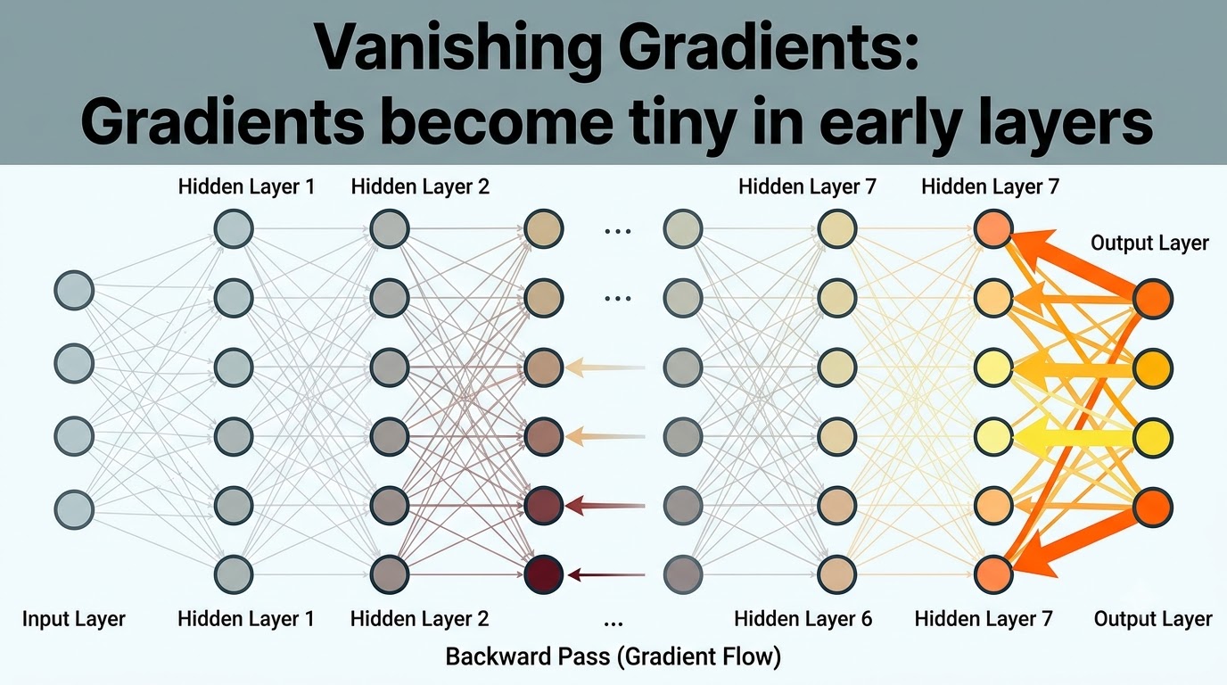
The vanishing gradient problem occurs when gradients become extremely small as they propagate backward through many layers of a deep neural network. This typically happens with activation functions like sigmoid or tanh, whose derivatives are very small over large input ranges. As these small derivatives are multiplied together layer by layer, the gradient signal diminishes rapidly.
When gradients vanish, the weight updates in the earlier layers of the network become negligible. This means that these initial layers learn very slowly, or sometimes stop learning altogether. Consequently, the network struggles to capture long-range dependencies in the data, impacting its overall performance.
This problem is particularly pronounced in recurrent neural networks (RNNs) when processing long sequences. It makes it challenging for the network to remember information from earlier time steps. Addressing vanishing gradients is a key area of research and practical application in deep learning.
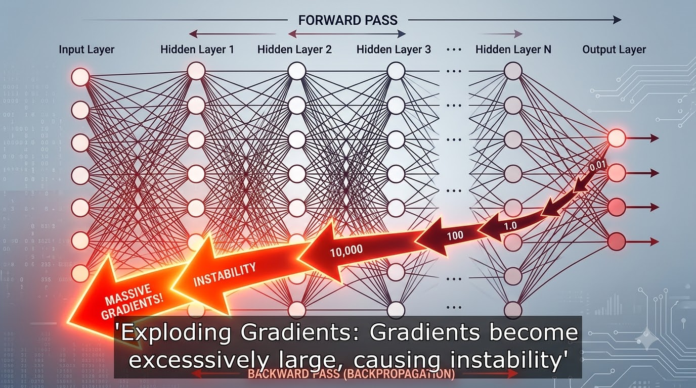
Conversely, the exploding gradient problem occurs when gradients become excessively large during backpropagation. This often happens in deep networks or recurrent neural networks, where the repeated multiplication of large gradients across layers can lead to an exponential increase in their magnitude. It's the opposite extreme of vanishing gradients.
When gradients explode, the weight updates become extremely large and unstable. This causes the model's parameters to change drastically with each iteration, preventing the optimization algorithm from converging. The network might oscillate wildly or even produce 'NaN' (Not a Number) values, indicating complete instability.
Exploding gradients make training very difficult, as the model cannot find a stable minimum for the loss function. This issue is particularly common in RNNs when dealing with long sequences. Techniques like gradient clipping are often employed to manage this problem effectively.
Beyond vanishing and exploding gradients, other challenges can impede backpropagation. Slow convergence is a common issue, where the model takes an inordinate amount of time to reach an optimal solution. This can be due to a poorly chosen learning rate, complex loss landscapes, or suboptimal network architecture.
Another significant problem is getting stuck in local minima. The loss function landscape for deep neural networks is often highly non-convex, meaning it has many dips and valleys. Gradient Descent might find a local minimum, which is a point where the loss is lower than its immediate surroundings, but not the absolute lowest point (global optimum).
While modern deep learning research suggests that for very high-dimensional spaces, local minima might not be as problematic as saddle points, the risk of suboptimal convergence remains. These issues highlight the importance of careful model design, hyperparameter tuning, and the use of advanced optimization techniques to navigate complex loss landscapes effectively.
To overcome the challenges of backpropagation and significantly improve training efficiency and stability, several advanced techniques have been developed. These methods are crucial for successfully training deep and complex neural networks. They address issues like slow convergence, vanishing/exploding gradients, and poor generalization.
These techniques range from smarter ways to initialize weights to sophisticated normalization layers and adaptive optimization algorithms. Implementing them correctly can dramatically reduce training time and lead to more robust models. They form the backbone of modern deep learning practices.
Understanding and applying these optimizations is a key skill for any deep learning practitioner. They allow models to learn faster, converge more reliably, and achieve higher performance on various tasks. Let's explore some of the most impactful techniques.
| Technique | Description | Benefit for Backpropagation |
|---|---|---|
| Better Weight Initialization | Initializing weights with small random values from specific distributions (e.g., Xavier/Glorot, He initialization). | Prevents gradients from vanishing or exploding early in training by keeping activations and gradients in a reasonable range. |
| Batch Normalization | Normalizing the inputs of each layer to have zero mean and unit variance during training. | Stabilizes learning, allows higher learning rates, reduces sensitivity to initialization, and acts as a regularizer. |
| Dropout | Randomly setting a fraction of neuron outputs to zero during training. | Prevents overfitting by forcing the network to learn more robust features and reducing co-adaptation of neurons. |
| Adaptive Optimizers (e.g., Adam, RMSprop) | Algorithms that adapt the learning rate for each parameter individually based on past gradients. | Accelerate convergence, handle sparse gradients, and often perform better than standard SGD, especially in complex landscapes. |
| Suitable Activation Functions | Choosing activation functions like ReLU, Leaky ReLU, or ELU instead of Sigmoid/Tanh for hidden layers. | Mitigate vanishing gradients by having non-zero derivatives over a wider range, speeding up learning. |
Backpropagation is not just an academic concept; it is the engine behind virtually every successful deep learning application we see today. Its ability to efficiently train complex neural networks has revolutionized numerous industries and fields. From everyday technology to cutting-edge research, its impact is pervasive.
In computer vision, backpropagation enables image recognition, object detection, and facial recognition systems. Natural language processing relies on it for tasks like language translation, sentiment analysis, and chatbots. Speech recognition, recommendation systems, and even autonomous vehicles all leverage backpropagation for their core learning capabilities.
Furthermore, in healthcare, it powers diagnostic tools and drug discovery, while in generative AI, it trains models to create realistic images, text, and other media. Backpropagation forms the fundamental training mechanism for the vast majority of deep learning models, making it indispensable to the advancement of AI.
While understanding the mathematical details of backpropagation is crucial, modern deep learning frameworks like TensorFlow and PyTorch abstract away much of the manual implementation. These frameworks provide automatic differentiation capabilities, meaning you don't have to manually derive and code the gradients for each layer.
The typical workflow involves defining your neural network architecture, specifying a loss function, and choosing an optimizer. During the training loop, you perform a forward pass, calculate the loss, and then simply call a method (e.g., .backward() in PyTorch or tape.gradient() in TensorFlow) to compute all necessary gradients automatically.
The optimizer then uses these computed gradients to update the model's parameters. This automation allows developers to focus on model design and experimentation rather than intricate calculus. Let's look at concise examples for both TensorFlow and PyTorch.
import tensorflow as tf

# 1. Define the model
model = tf.keras.Sequential([
    tf.keras.layers.Dense(10, activation='relu', input_shape=(784,)),
    tf.keras.layers.Dense(10, activation='softmax')
])

# 2. Define loss function and optimizer
loss_fn = tf.keras.losses.SparseCategoricalCrossentropy(from_logits=False)
optimizer = tf.keras.optimizers.Adam(learning_rate=0.001)

# Dummy data for demonstration
# In a real scenario, this would be loaded from a dataset
X_train = tf.random.normal((64, 784)) # Batch of 64 samples, 784 features
y_train = tf.random.uniform((64,), maxval=10, dtype=tf.int32) # 64 labels (0-9)

# 3. Training loop (one epoch for simplicity)
epochs = 1
for epoch in range(epochs):
    with tf.GradientTape() as tape:
        # Forward pass: Compute predictions
        logits = model(X_train, training=True)
        # Calculate loss
        loss_value = loss_fn(y_train, logits)

    # Backward pass: Compute gradients with respect to trainable variables
    # This is where backpropagation happens automatically
    gradients = tape.gradient(loss_value, model.trainable_variables)

    # Update weights using the optimizer
    optimizer.apply_gradients(zip(gradients, model.trainable_variables))

    print(f"Epoch {epoch+1, Loss: {loss_value.numpy():.4f")

print("TensorFlow training loop complete.")import torch
import torch.nn as nn
import torch.optim as optim
# 1. Define the model
class SimpleNN(nn.Module):
def _ᵢnit__(self):
super(SimpleNN, self)._ᵢnit__()
self.fc1 = nn.Linear(784, 10)
self.relu = nn.ReLU()
self.fc2 = nn.Linear(10, 10)
self.softmax = nn.Softmax(dim=1)
def forward(self, x):
x = self.fc1(x)
x = self.relu(x)
x = self.fc2(x)
x = self.softmax(x)
return x
model = SimpleNN()
# 2. Define loss function and optimizer
criterion = nn.CrossEntropyLoss()
optimizer = optim.Adam(model.parameters(), lr=0.001)
# Dummy data for demonstration
# In a real scenario, this would be loaded from a DataLoader
X_train = torch.randn(64, 784) # Batch of 64 samples, 784 features
y_train = torch.randint(0, 10, (64,)) # 64 labels (0-9)
# 3. Training loop (one epoch for simplicity)
epochs = 1
for epoch in range(epochs):
# Zero the parameter gradients
optimizer.zero_grad()
# Forward pass: Compute predictions
outputs = model(X_train)
# Calculate loss
loss = criterion(outputs, y_train)
# Backward pass: Compute gradients
# This is where backpropagation happens automatically
loss.backward()
# Update weights using the optimizer
optimizer.step()
print(f"Epoch {epoch+1, Loss: {loss.item():.4f")
print("PyTorch training loop complete.")Backpropagation's enduring popularity stems from several significant advantages that make it highly effective for training complex neural networks. Its core strength lies in its computational efficiency for gradient calculation. This efficiency is critical for training models with millions or even billions of parameters.
It enables high accuracy by systematically minimizing prediction errors, allowing networks to learn intricate patterns and generalize well to unseen data. The algorithm's scalability means it can be applied to diverse AI applications, from simple perceptrons to massive transformer models. This versatility has cemented its role as the standard.
Despite its origins decades ago, backpropagation remains the most widely used and successful learning algorithm for deep learning. Its foundational principles continue to drive advancements in artificial intelligence. Its robustness and adaptability are unmatched by other current training methods.
Despite its widespread success, backpropagation does come with certain limitations. One major concern is the computational cost, especially when training extremely large networks on massive datasets. The process of repeatedly calculating and propagating gradients can be very resource-intensive, requiring powerful hardware.
Another limitation is its heavy dependence on vast amounts of labeled data for supervised learning tasks. Acquiring and annotating such datasets can be expensive and time-consuming. This data dependency can be a bottleneck for many real-world applications where labeled data is scarce.
Backpropagation is also sensitive to hyperparameter tuning, such as the learning rate, batch size, and network architecture. Poor choices can lead to slow convergence or unstable training. Challenges associated with extremely deep architectures, like vanishing or exploding gradients, also persist, prompting researchers to explore alternative or complementary training methods to overcome these inherent constraints.
Beginners often encounter common pitfalls when implementing or training neural networks with backpropagation. One frequent mistake is choosing an inappropriate learning rate. A learning rate that is too high can cause the model to diverge, while one that is too low can lead to painfully slow convergence.
Neglecting data normalization is another common error. Input features should typically be scaled to a similar range (e.g., 0 to 1 or -1 to 1) to prevent some features from dominating the learning process. Using unsuitable activation functions for specific tasks, such as sigmoid in deep hidden layers, can exacerbate vanishing gradients.
Ignoring overfitting, where the model performs well on training data but poorly on unseen data, is also a critical mistake. Finally, misunderstanding the role of gradients or how they are computed can lead to incorrect implementations. Avoiding these pitfalls through careful data preprocessing, hyperparameter tuning, and architectural choices leads to more stable and effective model training.
Backpropagation is the cornerstone of modern deep learning, enabling neural networks to learn from data and continuously improve their predictions. By systematically calculating and propagating error gradients backward through the network, it facilitates gradient-based optimization. This iterative process allows models to minimize their loss functions and achieve remarkable accuracy.
From its foundational role in training simple feedforward networks to its adaptation in complex architectures like CNNs and RNNs, backpropagation's influence is undeniable. While challenges like vanishing gradients exist, advanced techniques and robust frameworks have made it more accessible and powerful than ever. It remains the gold standard for training deep learning models.
A deep understanding of backpropagation is not just theoretical knowledge; it's essential for mastering deep learning concepts, effectively debugging models, and building more advanced and robust AI systems. It empowers developers to unlock the full potential of artificial intelligence. Embrace backpropagation, and you'll unlock the secrets to neural network learning.
Backpropagation is an algorithm used to efficiently calculate the gradients of the loss function with respect to the weights and biases of a neural network. Gradient descent is an optimization algorithm that uses these calculated gradients to update the network's parameters, iteratively moving them in the direction that minimizes the loss function. Backpropagation provides the 'how much' each parameter contributes to the error, while gradient descent uses that information to perform the 'update'.
While backpropagation is primarily associated with supervised learning, where labeled data is available, its core mechanism of gradient calculation can be adapted for certain unsupervised learning tasks. For example, in autoencoders, backpropagation is used to train the network to reconstruct its input, minimizing a reconstruction loss without explicit labels. It's the gradient computation part that is versatile, even if the overall learning paradigm changes.
Researchers are exploring several alternatives, though none have fully replaced backpropagation for general deep learning tasks. These include equilibrium propagation, which draws inspiration from biological neural networks, and various forms of evolutionary algorithms or reinforcement learning methods that optimize network weights without explicit gradient calculations. Direct feedback alignment and other biologically plausible learning rules are also active areas of research, aiming to overcome some of backpropagation's limitations.
For recurrent neural networks (RNNs), backpropagation is adapted into an algorithm called Backpropagation Through Time (BPTT). BPTT essentially unrolls the RNN over time, treating each time step as a separate layer in a feedforward network. Gradients are then calculated and propagated backward through this unrolled network, accounting for the temporal dependencies and shared weights across time steps. This allows RNNs to learn from sequential data.
The Jacobian matrix plays a crucial theoretical role in understanding backpropagation. It represents the matrix of all first-order partial derivatives of a vector-valued function. In backpropagation, the chain rule is applied repeatedly, and each step involves multiplying Jacobian matrices (or vectors by Jacobian matrices) to propagate the error gradients backward through the network layers. While not explicitly computed as full matrices in practice for efficiency, the underlying mathematics relies on these Jacobian transformations.
Backpropagation is the fundamental training algorithm for Convolutional Neural Networks (CNNs) just as it is for standard feedforward networks. The key difference lies in how gradients are calculated for convolutional and pooling layers. For convolutional layers, gradients are computed through a process called 'convolutional backpropagation,' which involves convolving the error signal with the flipped kernel. For pooling layers, gradients are typically propagated to the location that contributed the maximum value (for max pooling) or distributed equally (for average pooling) during the forward pass.
Unravel Gradient Descent, the core optimization algorithm powering deep learning. Learn its mechanics, types, challenges, and real-world applications in AI
Master Artificial Neural Networks (ANNs) with this comprehensive guide covering core concepts, Python implementation, and real-world uses for all skill levels
Unlock advanced CNN power: explore ResNet, Inception, DenseNet, transfer learning, and optimization with practical code examples.